The logistic distribution

Intermediate Regression in R

Richie Cotton

Data Evangelist at DataCamp

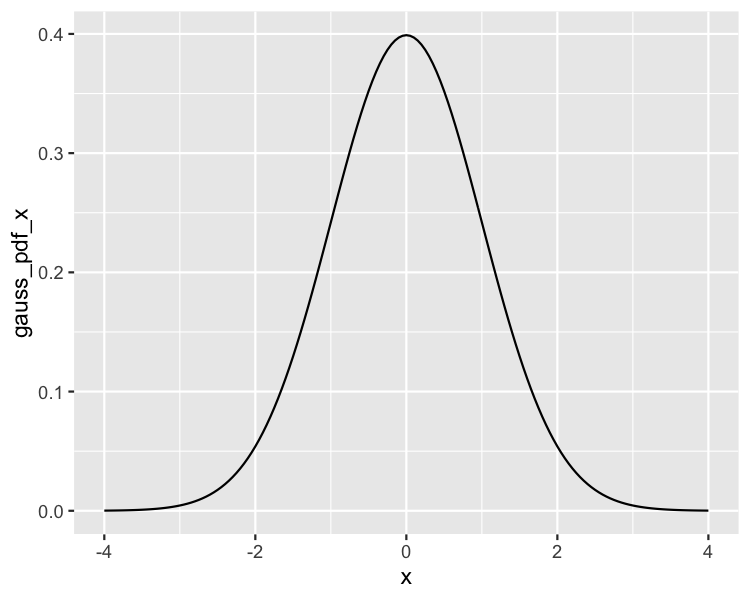
Gaussian probability density function (PDF)

gaussian_distn <- tibble(
  x = seq(-4, 4, 0.05),
  gauss_pdf_x = dnorm(x)
)

ggplot(gaussian_distn, aes(x, gauss_pdf_x)) +
  geom_line()

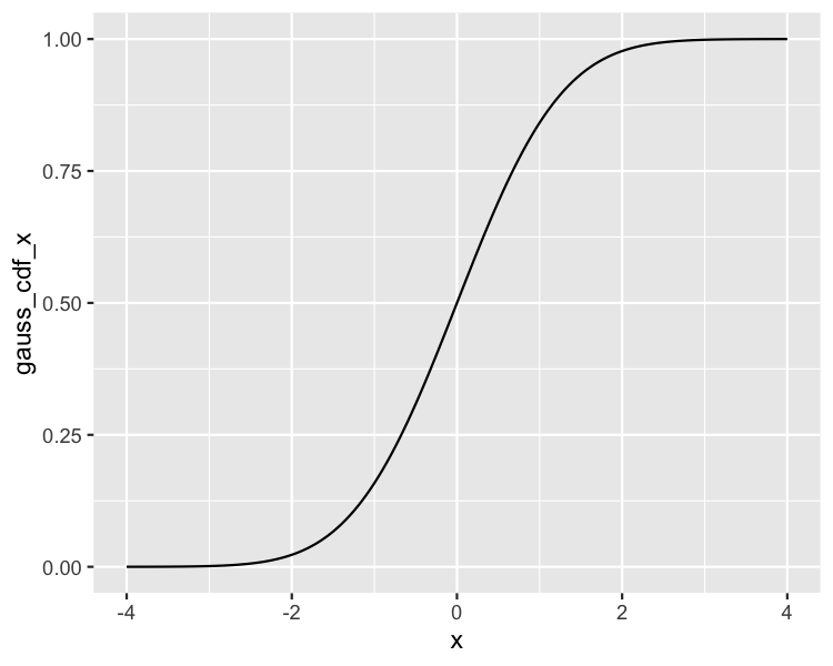
Gaussian cumulative distribution function (CDF)

gaussian_distn <- tibble(
  x = seq(-4, 4, 0.05),
  gauss_pdf_x = dnorm(x),
  gauss_cdf_x = pnorm(x)
)

ggplot(gaussian_distn, aes(x, gauss_cdf_x)) +
  geom_line()

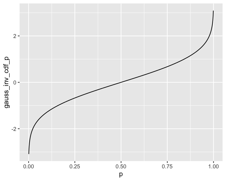
Gaussian inverse CDF

gaussian_distn_inv <- tibble(
  p = seq(0.001, 0.999, 0.001),
  gauss_inv_cdf_p = qnorm(p)
)

ggplot(gaussian_distn_inv, aes(p, gauss_inv_cdf_p)) +
  geom_line()

Distribution function names

curve	prefix	normal	logistic	nmemonic
PDF	d	`dnorm()`	`dlogis()`	"d" for differentiate - you differentiate the CDF to get the PDF
CDF	p	`pnorm()`	`plogis()`	"p" is backwards "q" so it's the inverse of the inverse CDF
Inv. CDF	q	`qnorm()`	`qlogis()`	"q" for quantile

glm()'s family argument

lm(response ~ explanatory, data = dataset)

glm(response ~ explanatory, data = dataset, family = gaussian)

glm(response ~ explanatory, data = dataset, family = binomial)

¹ https://campus.datacamp.com/courses/introduction-to-regression-in-r/simple-logistic-regression?ex=1

gaussian()

str(gaussian())

List of 11
 $ family    : chr "gaussian"
 $ link      : chr "identity"
 $ linkfun   :function (mu)  
 $ linkinv   :function (eta)  
 $ variance  :function (mu)  
 $ dev.resids:function (y, mu, wt)  
 $ aic       :function (y, n, mu, wt, dev)  
 $ mu.eta    :function (eta)  
 $ initialize:  expression({  n <- rep.int(1, nobs)  if (is.null(etastart) && is.null(start) &&
     is.null(mustart) &&  ((family$link| __truncated__
 $ validmu   :function (mu)  
 $ valideta  :function (eta)  
 - attr(*, "class")= chr "family"

linkfun and linkinv

Link function is a transformation of the response variable

gaussian()$linkfun

function (mu) 
mu

gaussian()$linkinv

function (eta) 
eta

Logistic PDF

logistic_distn <- tibble(
  x = seq(-6, 6, 0.05),
  logistic_pdf_x = dlogis(x)
)

ggplot(logistic_distn, aes(x, logistic_pdf_x)) +
  geom_line()

Logistic distribution

Logistic distribution CDF is also called the logistic function.
$\text{cdf}(x) = \frac{1}{(1 + exp(-x))}$
Logistic distribution inverse CDF is also called the logit function.
$\text{inverse\_cdf}(p) = log(\frac{p}{(1 - p)})$

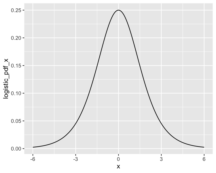
Let's practice!

Intermediate Regression in R