Continuing the infer pipeline

Hypothesis Testing in R

Richie Cotton

Data Evangelist at DataCamp

Recap: hypotheses and dataset

$H_{0}$: The proportion of hobbyists under 30 is the same as the prop'n of hobbyists at least 30.

$H_{A}$: The proportion of hobbyists under 30 is different from the prop'n of hobbyists at least 30.

alpha <- 0.1

stack_overflow_imbalanced %>% 
  count(hobbyist, age_cat, .drop = FALSE)

  hobbyist     age_cat    n
1       No At least 30    0
2       No    Under 30  191
3      Yes At least 30   15
4      Yes    Under 30 1025

Recap: workflow

null_distn <- dataset %>% 
  specify() %>% 
  hypothesize() %>% 
  generate() %>% 
  calculate()

observed_stat <- dataset %>% 
  specify() %>% 
  calculate()

get_p_value(null_distn, observed_stat)

stack_overflow_imbalanced %>%
  specify(hobbyist ~ age_cat, success = "Yes") %>% 
  hypothesize(null = "independence")

Response: hobbyist (factor)
Explanatory: age_cat (factor)
Null Hypothesis: independence
# A tibble: 1,231 x 2
  hobbyist age_cat    
  <fct>    <fct>      
1 Yes      At least 30
2 Yes      At least 30
3 Yes      At least 30
4 Yes      Under 30   
5 Yes      At least 30
6 Yes      At least 30
7 No       Under 30   
# ... with 1,224 more rows

Motivating generate()

$H_{0}$: The proportion of hobbyists under 30 is the same as the prop'n of hobbyists at least 30.

If $H_{0}$ is true, then

In each row, the hobbyist value could have appeared with either age category with equal probability.
To simulate this, we can permute (shuffle) the hobbyist values while keeping the age categories fixed.

stack_overflow_imbalanced

# A tibble: 1,231 x 2
  hobbyist age_cat    
  <fct>    <fct>      
1 Yes      At least 30
2 Yes      At least 30
3 Yes      At least 30
4 Yes      Under 30   
5 Yes      At least 30
6 Yes      At least 30
7 No       Under 30   
# ... with 1,224 more rows

bind_cols(
  stack_overflow_imbalanced %>% 
    select(hobbyist) %>% 
    slice_sample(prop = 1),
  stack_overflow_imbalanced %>% 
    select(age_cat)
)

# A tibble: 1,231 x 2
  hobbyist age_cat    
  <fct>    <fct>      
1 Yes      At least 30
2 Yes      At least 30
3 No       At least 30
4 No       Under 30   
5 Yes      At least 30
6 Yes      At least 30
7 Yes      Under 30   
# ... with 1,224 more rows

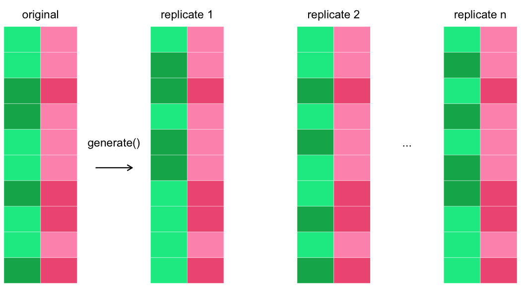
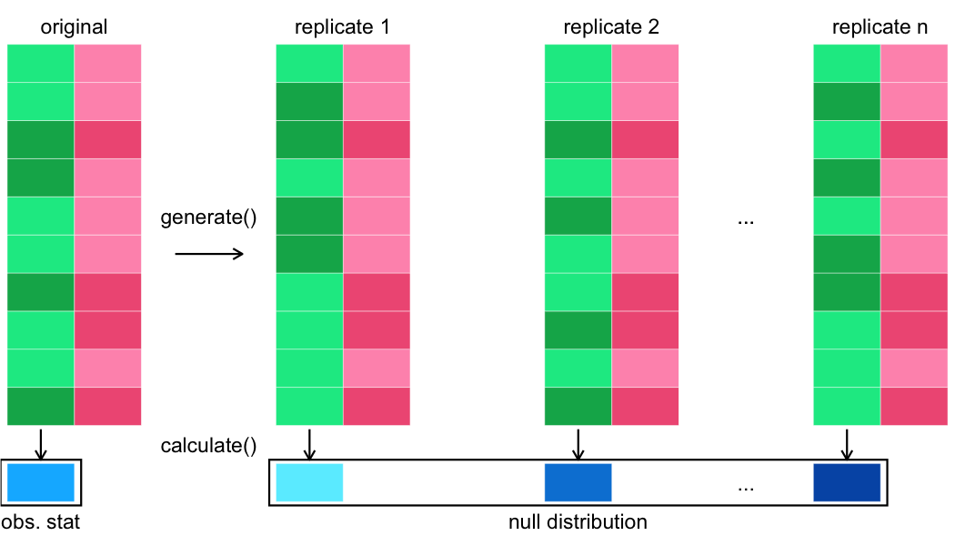
Generating many replicates

generate()

generate() generates simulated data reflecting the null hypothesis.

For "independence" null hypotheses, set type to "permute".
For "point" null hypotheses, set type to "bootstrap" or "simulate".

stack_overflow_imbalanced %>%
  specify(hobbyist ~ age_cat, success = "Yes") %>% 
  hypothesize(null = "independence") %>% 
  generate(reps = 5000, type = "permute")

Response: hobbyist (factor)
Explanatory: age_cat (factor)
Null Hypothesis: independence
# A tibble: 6,155,000 x 3
# Groups:   replicate [5,000]
  hobbyist age_cat     replicate
  <fct>    <fct>           <int>
1 Yes      At least 30         1
2 Yes      At least 30         1
3 Yes      At least 30         1
4 Yes      Under 30            1
5 Yes      At least 30         1
6 Yes      At least 30         1
7 Yes      Under 30            1
# ... with 6,154,993 more rows

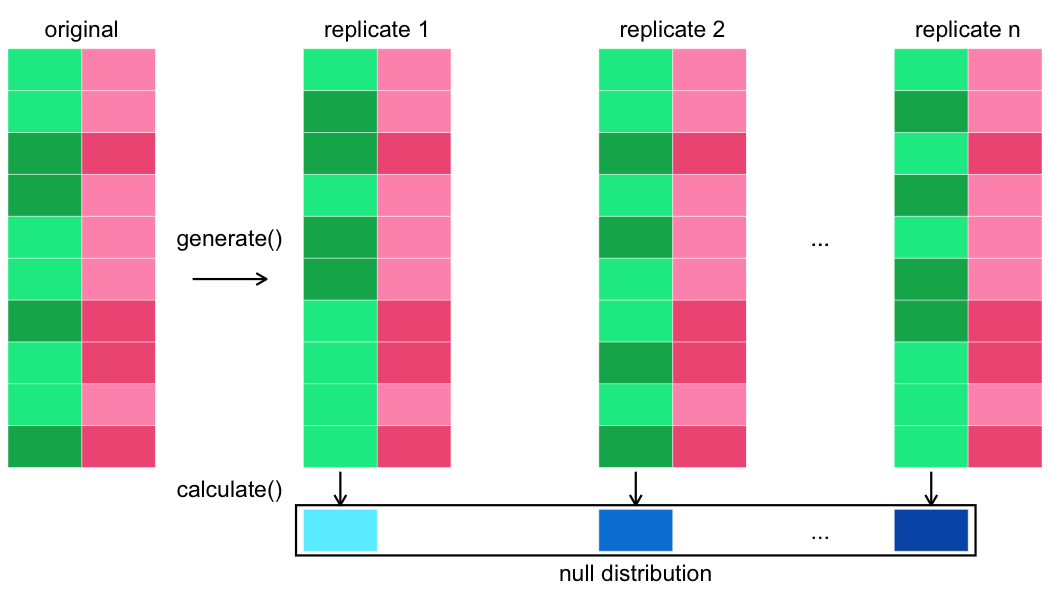
Calculating the test statistic

The rectangular grids representing the original dataset and replicates, that you saw in the generation step, are shown. Underneath these, the word 'calculate' is shown, and underneath each replicate is a downward arrow. Underneath each arrow is a single shaded cell representing a test statistic. A box is drawn around all the test statistics for the replicates, and labeled 'null distribution'.

calculate()

calculate() calculates a distribution of test statistics known as the null distribution.

null_distn <- stack_overflow_imbalanced %>%
  specify(
    hobbyist ~ age_cat, 
    success = "Yes"
  ) %>%
  hypothesize(null = "independence") %>%
  generate(reps = 5000, type = "permute") %>%
  calculate(
    stat = "diff in props", 
    order = c("At least 30", "Under 30")
  )

# A tibble: 5,000 x 2
  replicate    stat
      <int>   <dbl>
1         1  0.0896
2         2  0.0896
3         3 -0.180 
4         4  0.157 
5         5  0.0896
6         6 -0.113 
7         7  0.0221
# ... with 4,993 more rows

¹ The ?calculate help page lists all possible test statistics.

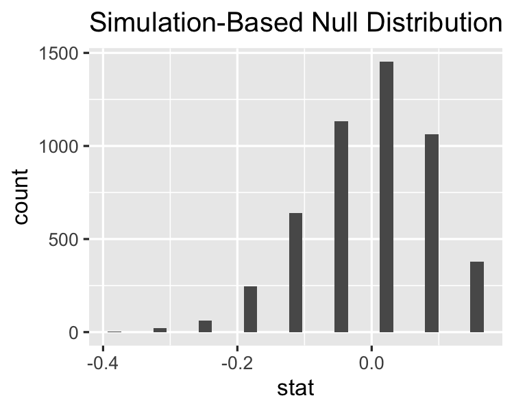
Visualizing the null distribution

visualize(null_distn)

A histogram of the null distribution. It is left-skewed, and there are nine distinct values.

null_distn %>% count(stat)

# A tibble: 9 x 2
     stat     n
    <dbl> <int>
1 -0.383      2
2 -0.315     22
3 -0.248     63
4 -0.180    246
5 -0.113    641
6 -0.0454  1132
7  0.0221  1453
8  0.0896  1063
9  0.157    378

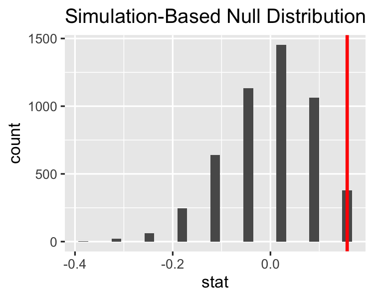
Calculating the test statistic on the original dataset

The rectangular grids representing the original dataset and replicates, along with the null distribution cells that you saw in the calculate step, are shown. This time, there is also a downward arrow below the original dataset, and underneath that, a shaded cell. This cell has a box around it labeled 'observed statistic'.

Observed statistic: specify() %>% calculate()

obs_stat <- stack_overflow_imbalanced %>%
  specify(hobbyist ~ age_cat, success = "Yes") %>%
  # hypothesize(null = "independence") %>%
  # generate(reps = 5000, type = "permute") %>%
  calculate(
    stat = "diff in props",
    order = c("At least 30", "Under 30")
  )

# A tibble: 1 x 1
   stat
  <dbl>
1 0.157

Visualizing the null distribution vs the observed stat

visualize(null_distn) +
  geom_vline(
    aes(xintercept = stat),
    data = observed_stat, 
    color = "red"
  )

The histogram of the null distribution, with an additional red vertical line at the observed statistic. The vertical line is over the right-most bar in the histogram.

Get the p-value

get_p_value(
  null_distn, obs_stat, 
  direction = "two sided"   # Not alternative = "two.sided"
)

# A tibble: 1 x 1
  p_value
    <dbl>
1   0.151

# A tibble: 1 x 6
  statistic chisq_df p_value alternative lower_ci upper_ci
      <dbl>    <dbl>   <dbl> <chr>          <dbl>    <dbl>
1      2.79        1  0.0949 two.sided    0.00718   0.0217

Let's practice!

Hypothesis Testing in R