Visualizing your Kaplan-Meier model

Survival Analysis in Python

Shae Wang

Senior Data Scientist

How to construct a Kaplan-Meier survival curve?

Toy data with $n=5$:

duration	observed
2	1
5	0
3	1
5	1
2	0

Step 1: Arrange data in increasing order. If tied, censored data comes after uncensored data.

Step 2: For each $t_i$, calculate $d_i$, $n_i$, and $\big(1-\frac{d_i}{n_i}\big)$

Step 3: For each $t_i$, multiply $\big(1-\frac{d_i}{n_i}\big)$ with $\big(1-\frac{d_{i-1}}{n_{i-1}}\big)$, $\big(1-\frac{d_{i-2}}{n_{i-2}}\big)$, ... , $\big(1-\frac{d_0}{n_0}\big)$

How to construct a Kaplan-Meier survival curve?

Step 1: Arrange durations in increasing order. If tied, censored data comes after uncensored data.

duration
2
5+
3
5
2+

Use "+" sign to denote censored data: 2, 5+, 3, 5, 2+

How to construct a Kaplan-Meier survival curve?

Step 1: Arrange durations in increasing order. If tied, censored data comes after uncensored data.

$t_i$
2, 2+
3
5, 5+

How to construct a Kaplan-Meier survival curve?

Step 2: For each $t_i$, calculate $d_i$, $n_i$, and $\big(1-\frac{d_i}{n_i}\big)$

$t_i$
2, 2+
3
5, 5+

How to construct a Kaplan-Meier survival curve?

Step 2: For each $t_i$, calculate $d_i$, $n_i$, and $\big(1-\frac{d_i}{n_i}\big)$

$t_i$	$d_i$
2, 2+	1
3	1
5, 5+	1

How to construct a Kaplan-Meier survival curve?

Step 2: For each $t_i$, calculate $d_i$, $n_i$, and $\big(1-\frac{d_i}{n_i}\big)$

$t_i$	$d_i$	$n_i$
2, 2+	1	5
3	1	3
5, 5+	1	2

How to construct a Kaplan-Meier survival curve?

Step 2: For each $t_i$, calculate $d_i$, $n_i$, and $\big(1-\frac{d_i}{n_i}\big)$

$t_i$	$d_i$	$n_i$	$\big(1-\frac{d_i}{n_i}\big)$
2, 2+	1	5	$4/5$
3	1	3	$2/3$
5, 5+	1	2	$1/2$

How to construct a Kaplan-Meier survival curve?

Step 3: For each $t_i$, multiply $\big(1-\frac{d_i}{n_i}\big)$ with $\big(1-\frac{d_{i-1}}{n_{i-1}}\big)$, $\big(1-\frac{d_{i-2}}{n_{i-2}}\big)$, ... , $\big(1-\frac{d_0}{n_0}\big)$

$t_i$	$d_i$	$n_i$	$\big(1-\frac{d_i}{n_i}\big)$	$S(t_i)$
2, 2+	1	5	4/5	4/5 = 0.8
3	1	3	2/3	4/5 $\cdot$ 2/3 = 0.53
5, 5+	1	2	1/2	4/5 $\cdot$ 2/3 $\cdot$ 1/2 = 0.27

How to construct a Kaplan-Meier survival curve?

$t_i$	$d_i$	$n_i$	$\big(1-\frac{d_i}{n_i}\big)$	$S(t_i)$
2, 2+	1	5	$4/5$	0.8
3	1	3	$2/3$	0.53
5, 5+	1	2	$1/2$	0.27

Kaplan-Meier curve from table.

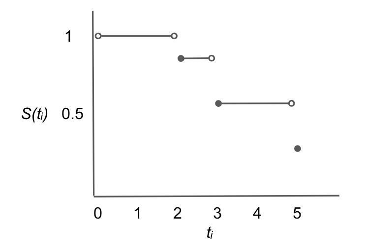
Interpreting the survival curve

Kaplan-Meier curve from table.

The survival probabilities at each time between 0 and 5.
Common misconception: If the curve goes to 0, no subjects survived.
The curve will drop to zero if the last observation is not censored (true event duration is known).

Plotting the Kaplan-Meier survival curve

from lifelines import KaplanMeierFitter
import matplotlib.pyplot as plt

kmf = KaplanMeierFitter()
kmf.fit(durations, event_observed)

kmf.survival_function_.plot()
plt.show()

The mortgage problem example

DataFrame name: mortgage_df

id	duration	paid_off
1	25	0
2	17	1
3	5	0
...	...	...
100	30	1

from lifelines import KaplanMeierFitter
from matplotlib import pyplot as plt

mortgage_kmf = KaplanMeierFitter()
mortgage_kmf.fit(duration=mortgage_df["duration"], 
        event_observed=mortgage_df["paid_off"])

mortgage_kmf.survival_function_.plot()

The mortgage problem example

plt.show()

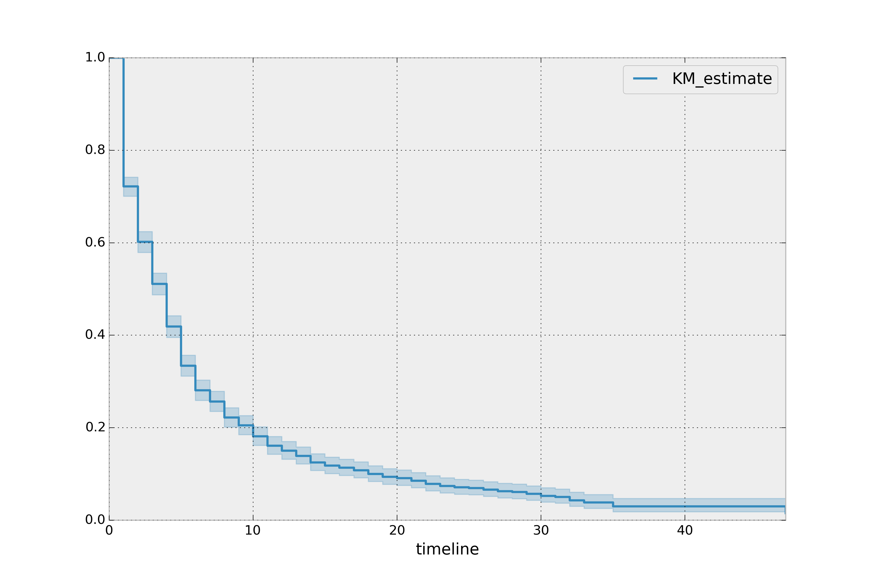
Mortgage problem survival curve visualization.

Survival curve confidence interval

mortgage_kmf.plot_survival_function()
plt.show()

Mortgage problem survival curve visualization with confidence interval.

Why is the confidence interval useful?

A way to quantify how uncertain we are about each point estimate of survival probabilities
A wide confidence interval means we are less certain, often due to small sample size
A narrow confidence interval means we are more certain, often due to large sample size

Ways to plot the Kaplan-Meier survival curve

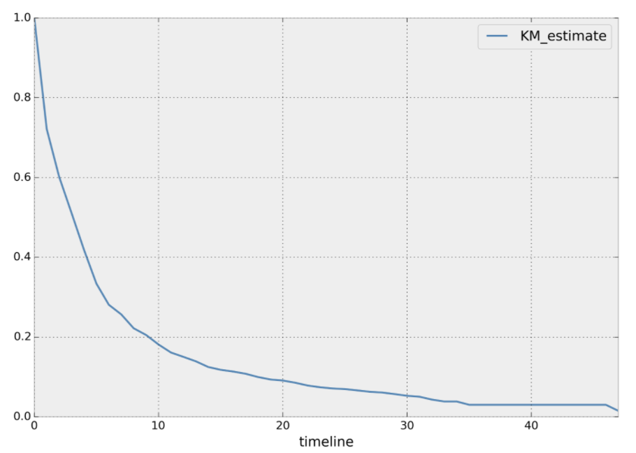
Plot survival function point estimates as a continuous line.

kmf.survival_function_.plot()
plt.show()

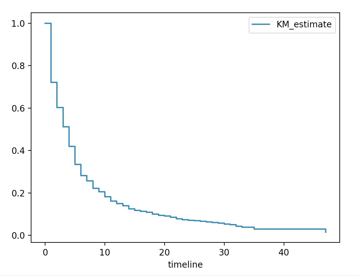
Survival function plot as a continuous line.

Plot survival function as a stepped line without the confidence interval.

kmf.plot(ci_show=False)
plt.show()

Survival function plot as a stepped line.

Ways to plot the Kaplan-Meier survival curve

Plot survival function as a stepped line with the confidence interval.

kmf.plot()
plt.show()

Survival function plot as a stepped line with confidence interval.

Another way...

kmf.plot_survival_function()
plt.show()

Let's practice!

Survival Analysis in Python