Gráficos de linhas
Introdução à Visualização de Dados com ggplot2

Rick Scavetta
Founder, Scavetta Academy
Castor
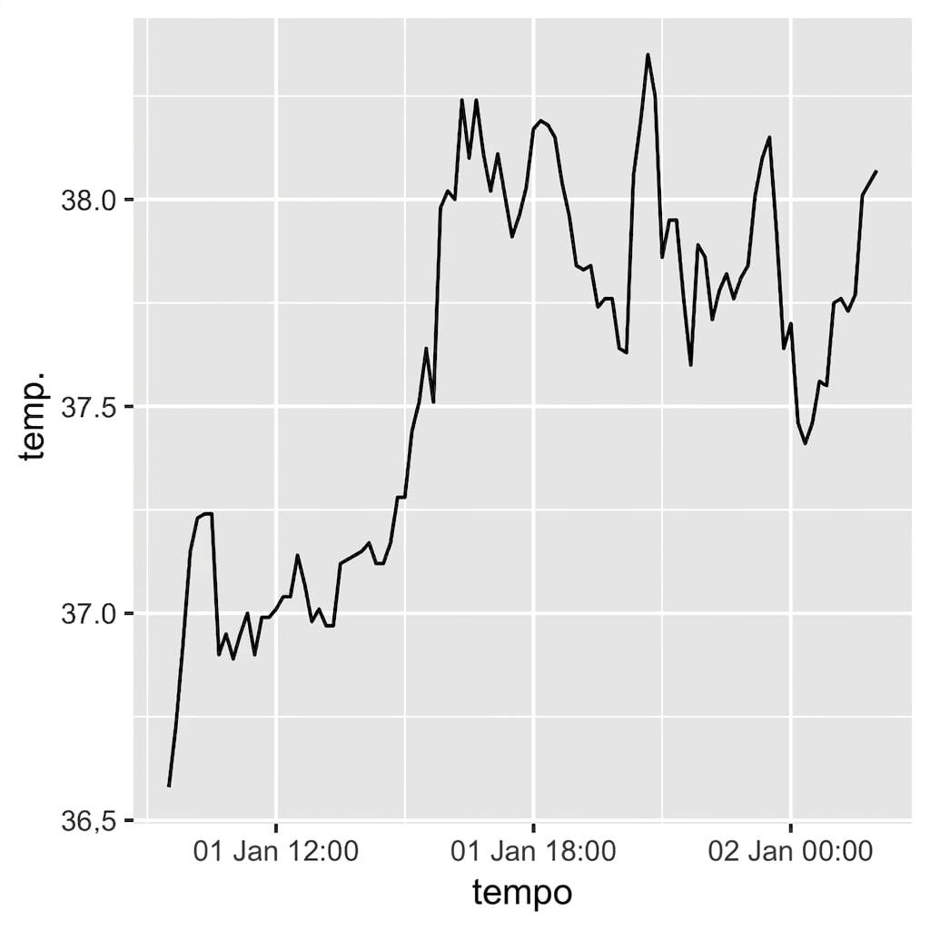
Castor
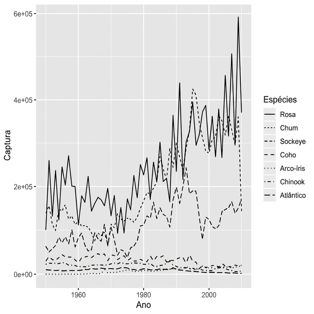
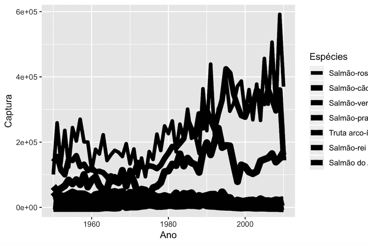
Estética linetype
Estética size
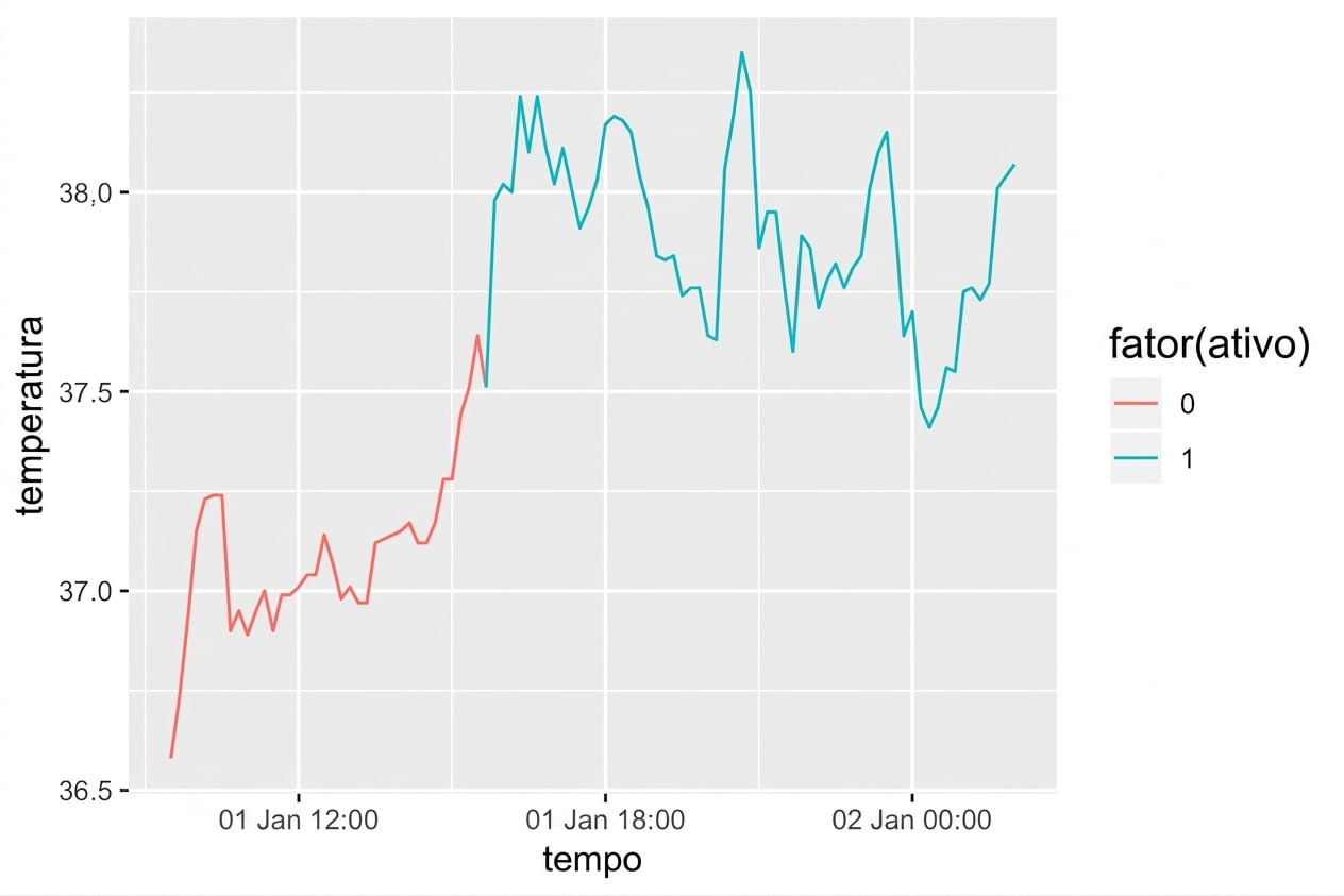
Estética color
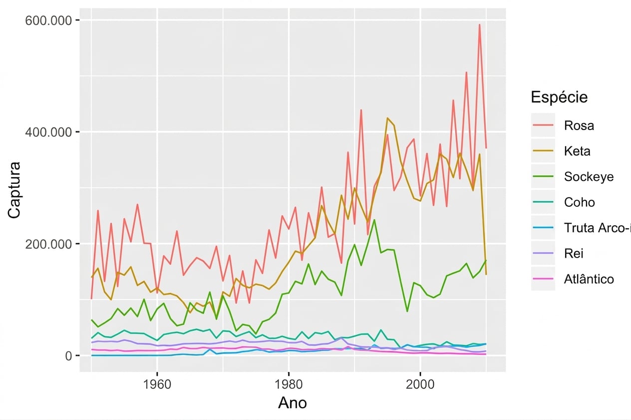
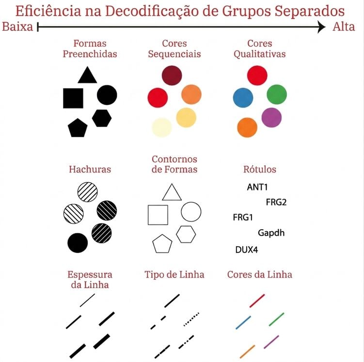
Estéticas para variáveis categóricas
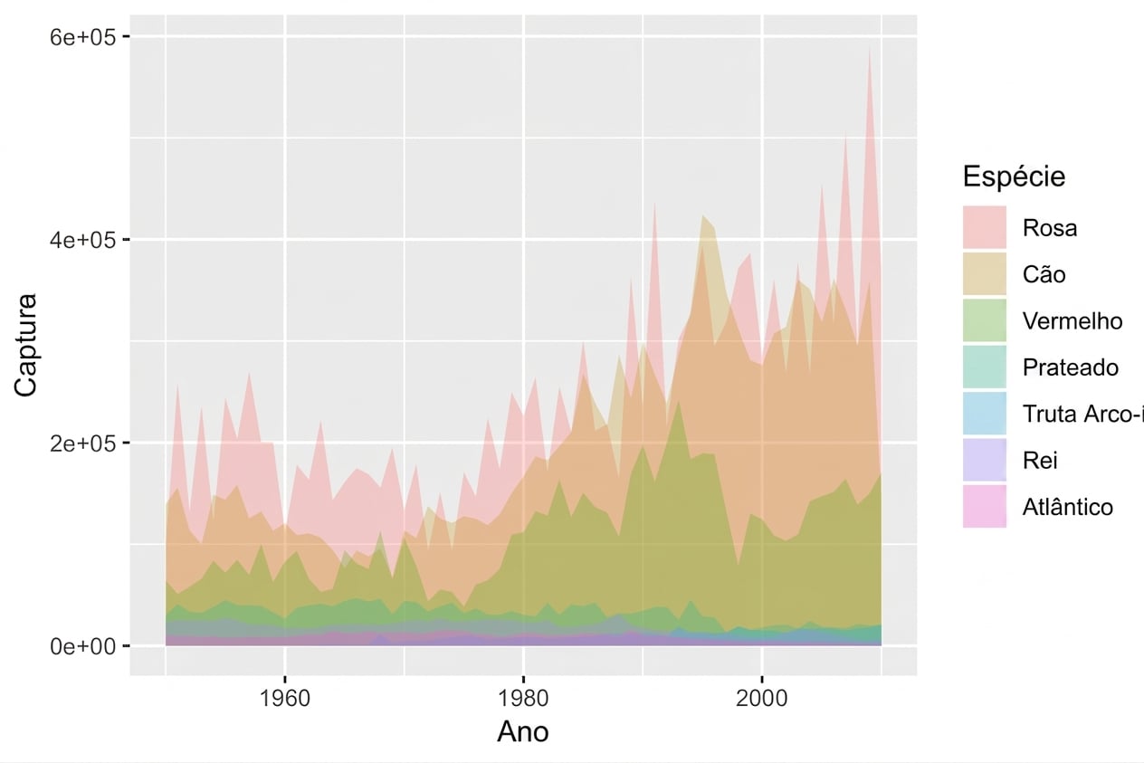
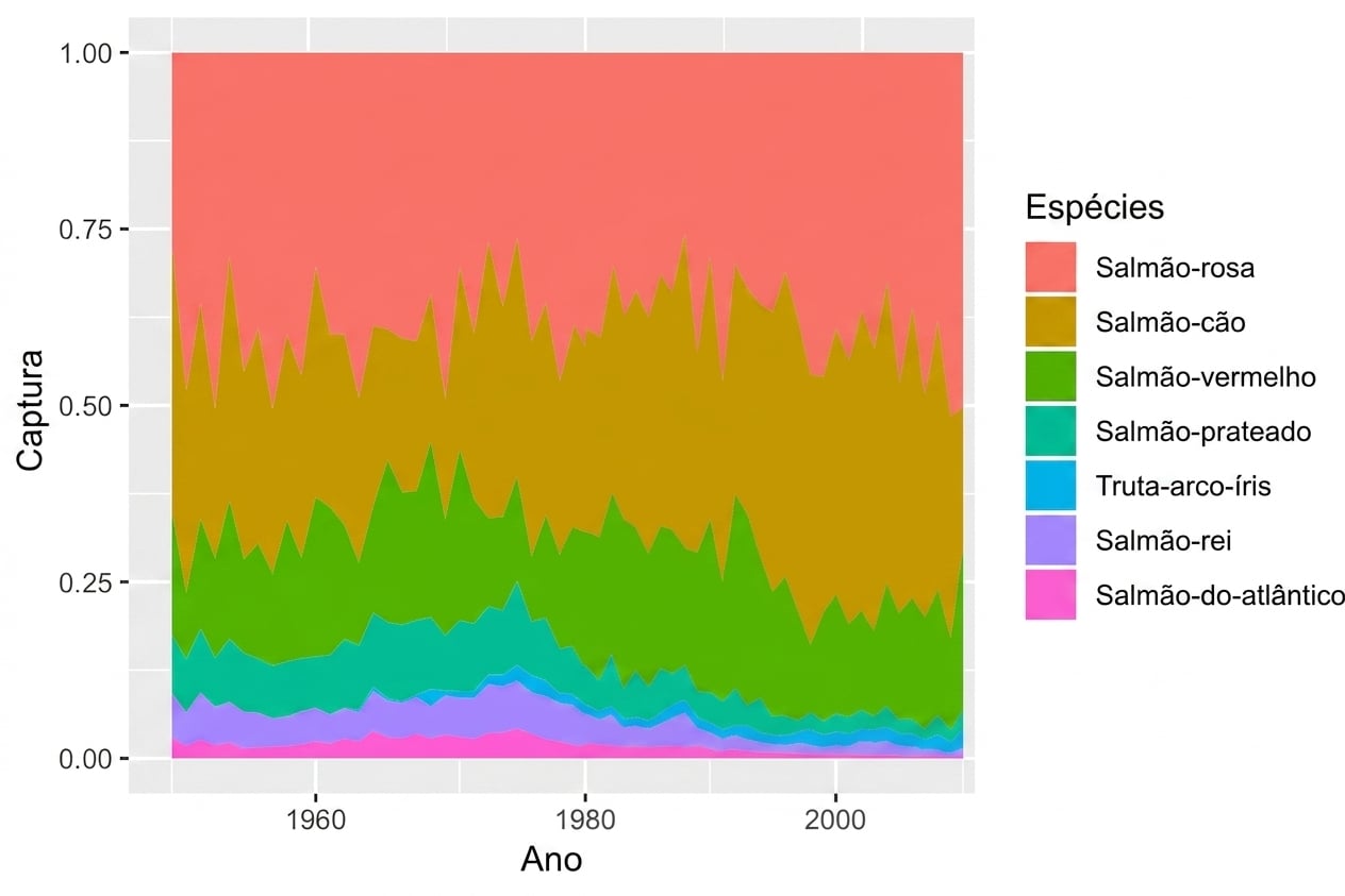
Preencher a estética com geom_area()
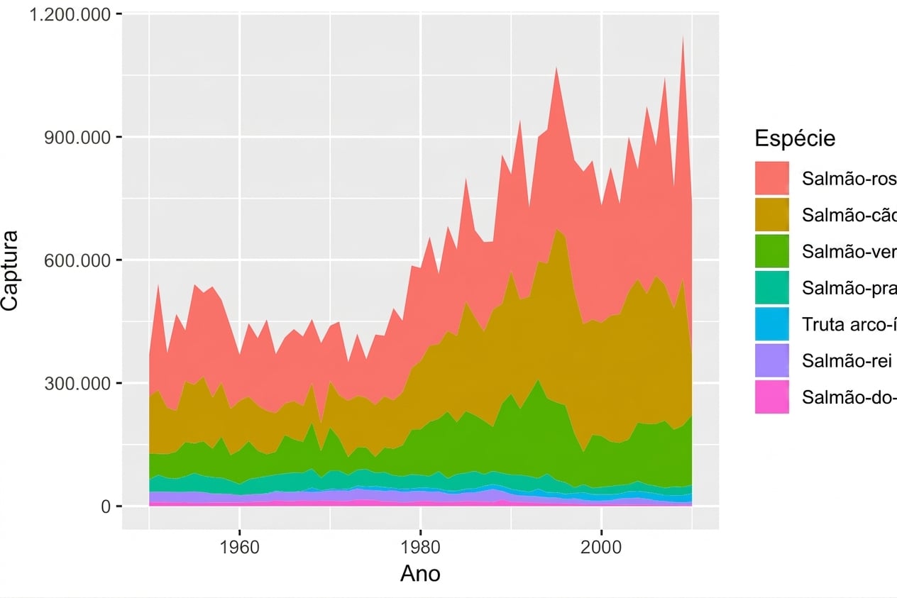
Uso de position = "fill"
geom_ribbon()