Medidas de tendência central
Introdução à Estatística em R

Maggie Matsui
Content Developer, DataCamp
Histogramas
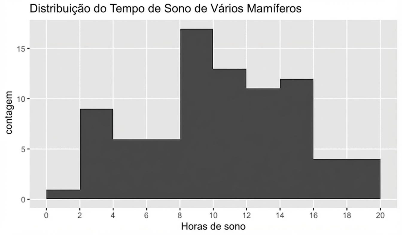
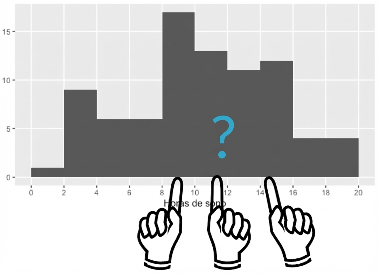
Quanto os mamíferos deste conjunto normalmente dormem?
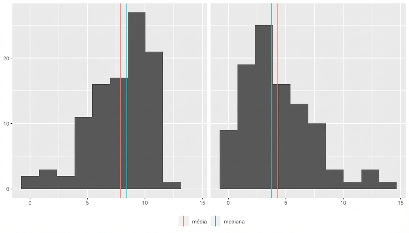
Qual medida usar?
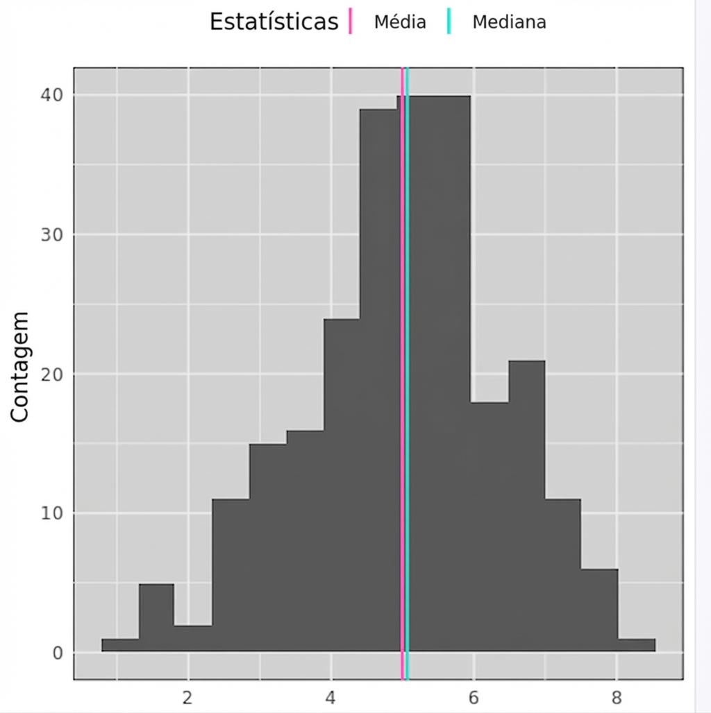
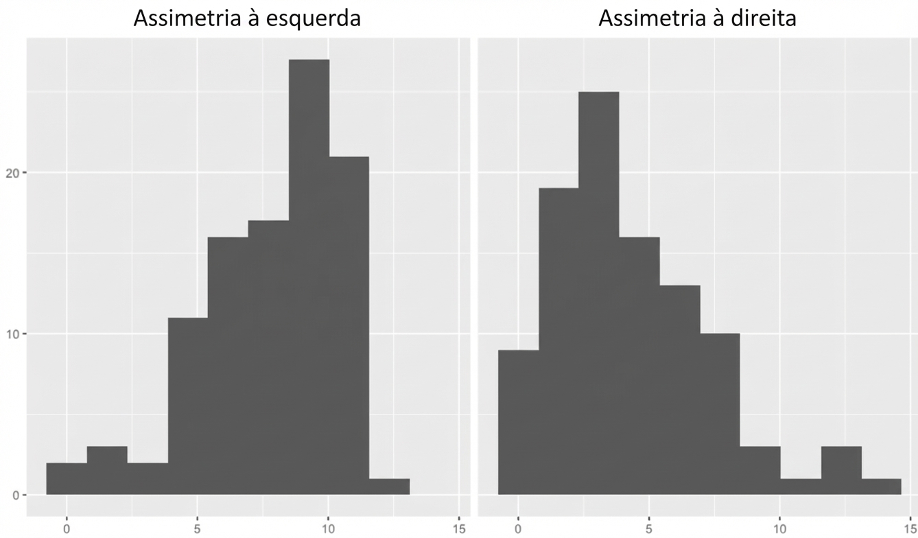
Assimetria
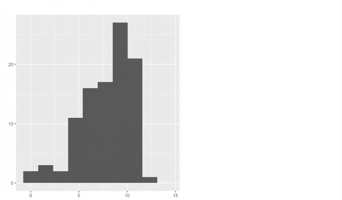
Assimetria

Assimetria
Qual medida usar?
Introdução à Estatística em R
Maggie Matsui
Content Developer, DataCamp

