Transformando variáveis

Introdução à Regressão em R

Richie Cotton

Data Evangelist at DataCamp

Conjunto de dados: perca

library(dplyr)

perch <- fish %>%
  filter(species == "Perch")

species	mass_g	length_cm
Perch	5.9	7.5
Perch	32.0	12.5
Perch	40.0	13.8
Perch	51.5	15.0
Perch	70.0	15.7
...	...	...

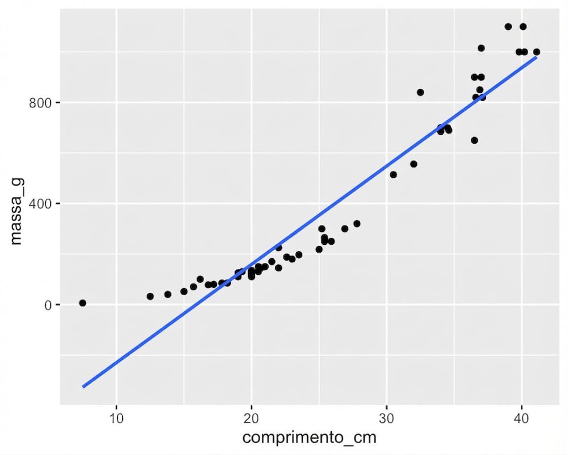
Não é relação linear

ggplot(perch, aes(length_cm, mass_g)) +
  geom_point() +
  geom_smooth(method = "lm", se = FALSE)

Dispersão da massa do perca vs. comprimento, com linha de tendência. A massa cresce mais rápido que linearmente com o comprimento, formando uma curva ascendente.

Bream vs. perca

Várias breamas nadando. Breams são bem achatadas.

Vários percas nadando. Percas são mais arredondadas.

Gráfico: massa vs. comprimento³

ggplot(perch, aes(length_cm ^ 3, mass_g)) +
  geom_point() +
  geom_smooth(method = "lm", se = FALSE)

Dispersão da massa do perca vs. comprimento ao cubo, com linha de tendência. Após a transformação, os pontos ficam perto da linha.

Modelando: massa vs. comprimento³

mdl_perch <- lm(mass_g ~ I(length_cm ^ 3), data = perch)

Call:
lm(formula = mass_g ~ I(length_cm^3), data = perch)

Coefficients:
   (Intercept)  I(length_cm^3)  
       -0.1175          0.0168

Prevendo: massa vs. comprimento³

explanatory_data <- tibble(
  length_cm = seq(10, 40, 5)
)

prediction_data <- explanatory_data %>%
  mutate(
    mass_g = predict(mdl_perch, explanatory_data)
  )

# A tibble: 7 x 2
  length_cm mass_g
      <dbl>  <dbl>
1        10   16.7
2        15   56.6
3        20  134. 
4        25  262. 
5        30  453. 
6        35  720. 
7        40 1075.

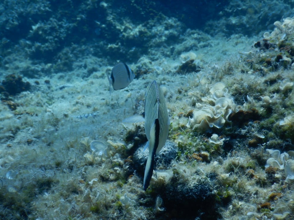
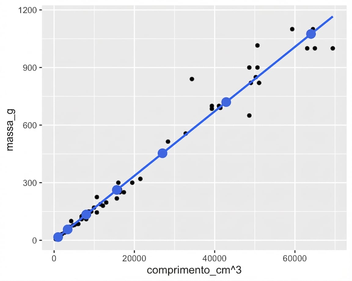
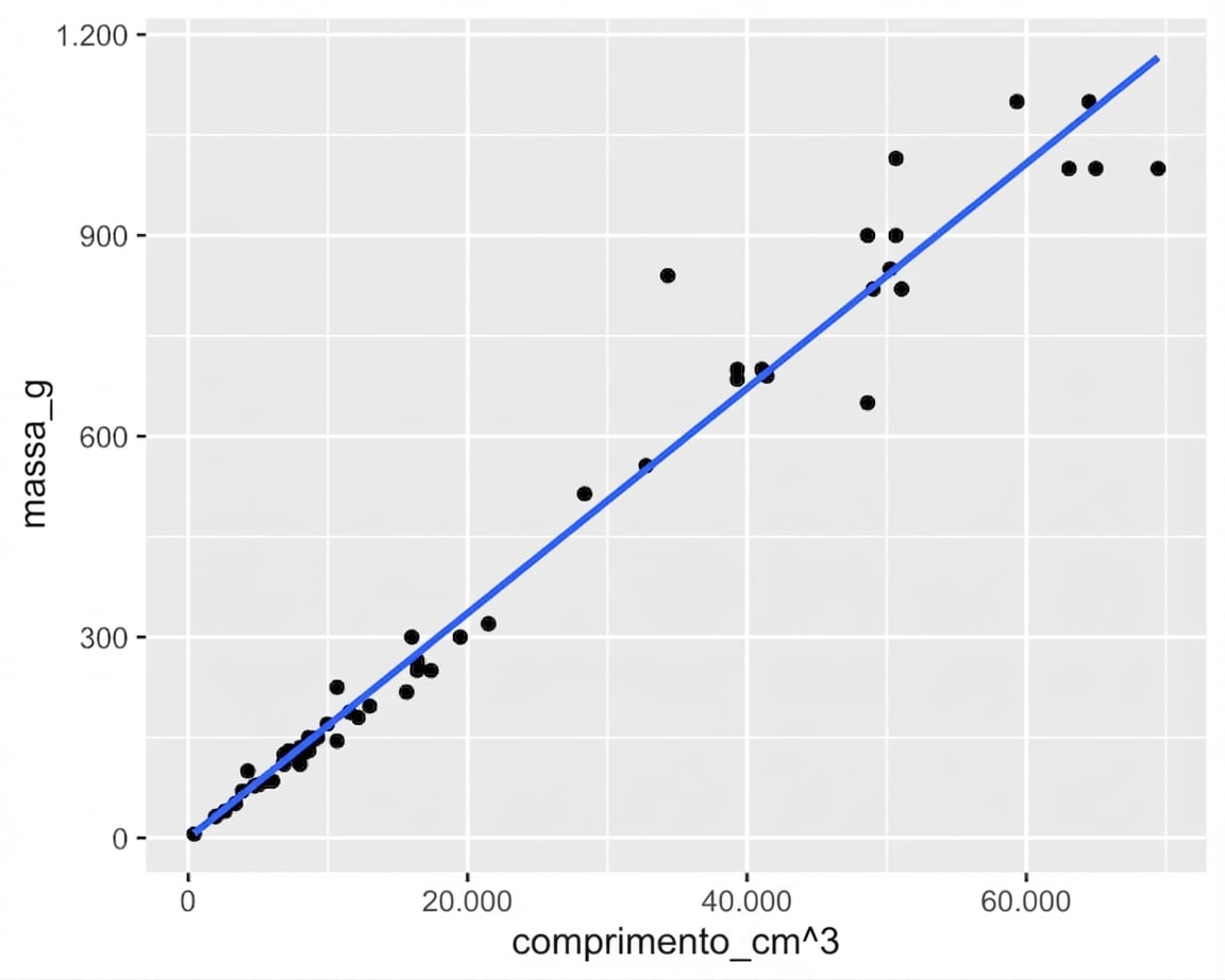
Gráfico: massa vs. comprimento³

ggplot(perch, aes(length_cm ^ 3, mass_g)) +
  geom_point() +
  geom_smooth(method = "lm", se = FALSE) +
  geom_point(data = prediction_data, color = "blue")

Dispersão da massa do perca vs. comprimento³, com linha de tendência, anotada com pontos do predict(). Eles seguem a linha exatamente.

ggplot(perch, aes(length_cm, mass_g)) +
  geom_point() +
  geom_smooth(method = "lm", se = FALSE) +
  geom_point(data = prediction_data, color = "blue")

Dispersão da massa do perca vs. comprimento, com linha de tendência, anotada com pontos do predict(). Eles não seguem a linha, mas acompanham a curvatura dos dados.

Conjunto: anúncios no Facebook

Como funciona a publicidade

Você paga o Facebook para mostrar anúncios.
As pessoas veem os anúncios ("impressões").
Algumas pessoas clicam.

936 linhas
Cada linha é 1 anúncio

spent_usd	n_impressions	n_clicks
1.43	7350	1
1.82	17861	2
1.25	4259	1
1.29	4133	1
4.77	15615	3
...	...	...

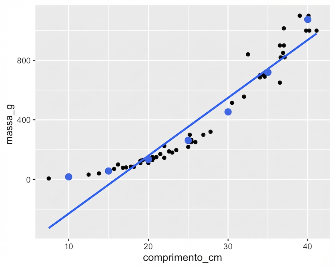
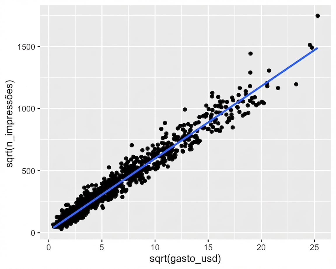
Gráfico apertado

ggplot(
  ad_conversion, 
  aes(spent_usd, n_impressions)
) +
  geom_point() +
  geom_smooth(method = "lm", se = FALSE)

Dispersão de impressões vs. gasto, com linha de tendência. A maioria dos pontos fica espremida no canto inferior esquerdo.

Raiz vs. raiz

ggplot(
  ad_conversion, 
  aes(sqrt(spent_usd), sqrt(n_impressions))
) +
  geom_point() +
  geom_smooth(method = "lm", se = FALSE)

Dispersão da raiz quadrada das impressões vs. raiz quadrada do gasto, com linha de tendência. Agora os pontos estão mais distribuídos.

Modelando e prevendo

mdl_ad <- lm(
  sqrt(n_impressions) ~ sqrt(spent_usd), 
  data = ad_conversion
)

explanatory_data <- tibble(
  spent_usd = seq(0, 600, 100)
)

prediction_data <- explanatory_data %>% 
  mutate(
    sqrt_n_impressions = predict(
      mdl_ad, explanatory_data
    ),
    n_impressions = sqrt_n_impressions ^ 2
  )

# A tibble: 7 x 3
  spent_usd sqrt_n_impressions n_impressions
      <dbl>              <dbl>         <dbl>
1         0               15.3          235.
2       100              598.        357289.
3       200              839.        703890.
4       300             1024.       1048771.
5       400             1180.       1392762.
6       500             1318.       1736184.
7       600             1442.       2079202.

Vamos praticar!

Introdução à Regressão em R