Quantificando o ajuste da regressão logística
Introdução à Regressão em R

Richie Cotton
Data Evangelist at DataCamp
Quatro possíveis resultados
| falso real | verdadeiro real | |
|---|---|---|
| previsto falso | correto | falso negativo |
| previsto verdadeiro | falso positivo | correto |
Matriz de confusão: contagem dos resultados
mdl_recency <- glm(has_churned ~ time_since_last_purchase, data = churn, family = "binomial")
actual_response <- churn$has_churned
predicted_response <- round(fitted(mdl_recency))
outcomes <- table(predicted_response, actual_response)
                  actual_response
predicted_response   0   1
                 0 141 111
                 1  59  89
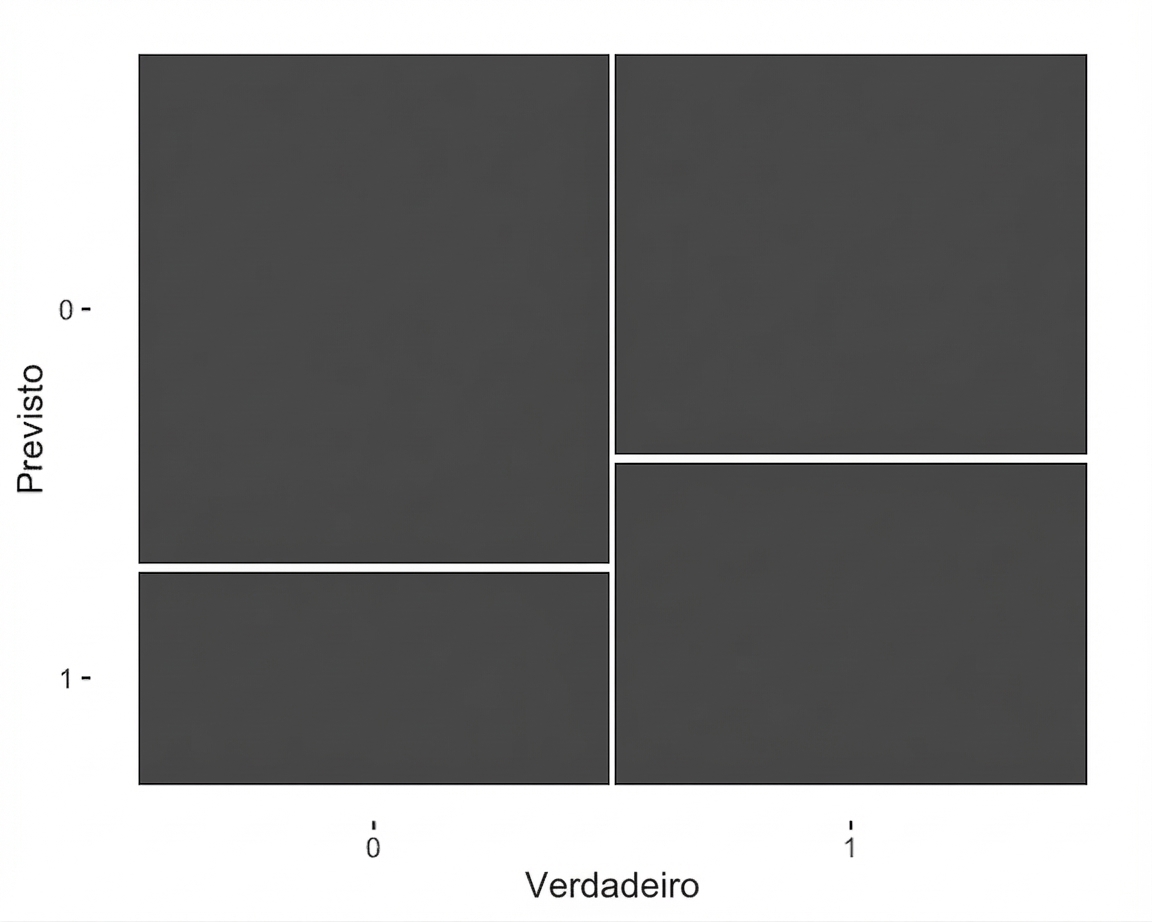
Visualizando a matriz de confusão: gráfico mosaico
library(ggplot2)
library(yardstick)
confusion <- conf_mat(outcomes)
                  actual_response
predicted_response   0   1
                 0 141 111
                 1  59  89
autoplot(confusion)
Métricas de desempenho
summary(confusion, event_level = "second")
# A tibble: 13 x 3
   .metric              .estimator .estimate
   <chr>                <chr>          <dbl>
 1 accuracy             binary         0.575
 2 kap                  binary         0.150
 3 sens                 binary         0.445
 4 spec                 binary         0.705
 5 ppv                  binary         0.601
 6 npv                  binary         0.560
 7 mcc                  binary         0.155
 8 j_index              binary         0.150
 9 bal_accuracy         binary         0.575
10 detection_prevalence binary         0.37
11 precision            binary         0.601
12 recall               binary         0.445
13 f_meas               binary         0.511
Acurácia
summary(confusion) %>%
  slice(1)
# A tibble: 3 x 3
  .metric  .estimator .estimate
  <chr>    <chr>          <dbl>
1 accuracy binary         0.575
Acurácia é a proporção de previsões corretas.
$$ accuracy = \frac{TN + TP}{TN + FN + FP + TP} $$
confusion
                  actual_response
predicted_response   0   1
                 0 141 111
                 1  59  89
(141 + 89) / (141 + 111 + 59 + 89)
0.575
Sensibilidade
summary(confusion) %>%
  slice(3)
# A tibble: 1 x 3
  .metric .estimator .estimate
  <chr>   <chr>          <dbl>
1 sens    binary         0.445
Sensibilidade é a proporção de verdadeiros positivos.
$$ sensitivity = \frac{TP}{FN + TP} $$
confusion
                  actual_response
predicted_response   0   1
                 0 141 111
                 1  59  89
89 / (111 + 89)
0.445
Especificidade
summary(confusion) %>%
  slice(4)
# A tibble: 1 x 3
  .metric .estimator .estimate
  <chr>   <chr>          <dbl>
1 spec    binary         0.705
Especificidade é a proporção de verdadeiros negativos.
$$ specificity = \frac{TN}{TN + FP} $$
confusion
                  actual_response
predicted_response   0   1
                 0 141 111
                 1  59  89
141 / (141 + 59)
0.705
Vamos praticar!
Introdução à Regressão em R

