Quantificando o ajuste do modelo

Introdução à Regressão em R

Richie Cotton

Data Evangelist at DataCamp

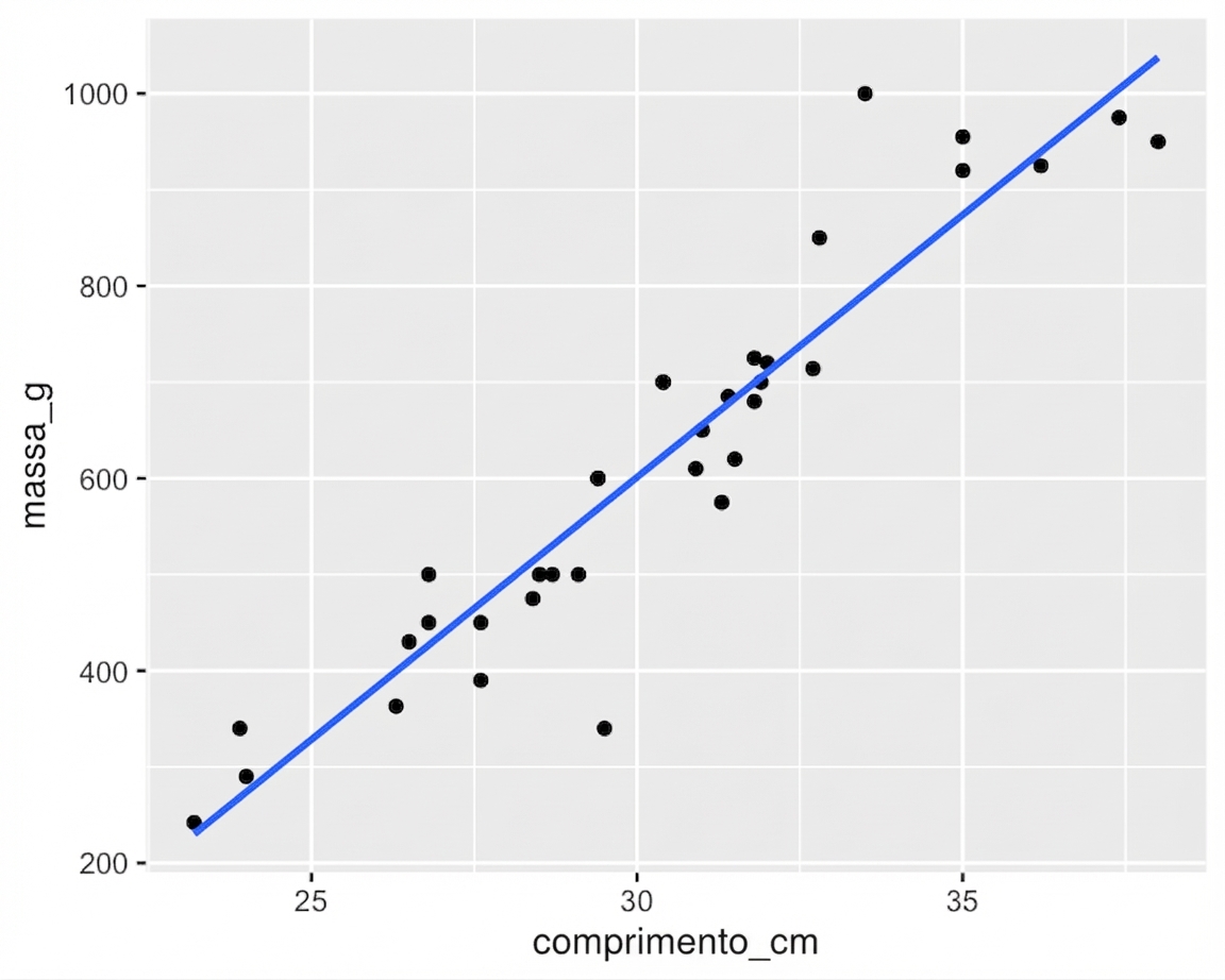
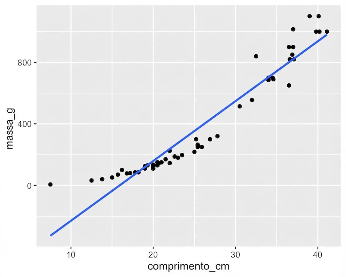
Modelos de bream e perca

Bream

O diagrama de dispersão das massas de bream versus seus comprimentos, com uma linha de tendência, mostrado antes.

Perch

O diagrama de dispersão das massas de perca versus seus comprimentos, com uma linha de tendência, mostrado antes.

Coeficiente de determinação

Também chamado de "r-quadrado" ou "R-quadrado".

a proporção da variância na variável resposta que é previsível pela variável explicativa

1 indica ajuste perfeito
0 indica pior ajuste possível

summary()

Veja o valor "Multiple R-Squared"

mdl_bream <- lm(mass_g ~ length_cm, data = bream)

summary(mdl_bream)

# Algumas linhas do output omitidas

Residual standard error: 74.15 on 33 degrees of freedom
Multiple R-squared:  0.8781,    Adjusted R-squared:  0.8744 
F-statistic: 237.6 on 1 and 33 DF,  p-value: < 2.2e-16

glance()

library(broom)
library(dplyr)
mdl_bream %>% 
  glance()

# A tibble: 1 × 12
  r.squared adj.r.squared sigma statistic  p.value    df logLik   AIC   BIC
      <dbl>         <dbl> <dbl>     <dbl>    <dbl> <dbl>  <dbl> <dbl> <dbl>
1     0.878         0.874  74.2      238. 1.22e-16     1  -199.  405.  409.
# ... with 3 more variables: deviance <dbl>, df.residual <int>, nobs <int>

mdl_bream %>% 
  glance() %>% 
  pull(r.squared)

0.8780627

É só a correlação ao quadrado

bream %>% 
  summarize(
    coeff_determination = cor(length_cm, mass_g) ^ 2
  )

  coeff_determination
1           0.8780627

Erro padrão residual (RSE)

uma diferença “típica” entre a predição e a resposta observada

Tem a mesma unidade da variável resposta.

summary() de novo

Veja o valor "Residual standard error"

summary(mdl_bream)

# Algumas linhas do output omitidas

Residual standard error: 74.15 on 33 degrees of freedom
Multiple R-squared:  0.8781,    Adjusted R-squared:  0.8744 
F-statistic: 237.6 on 1 and 33 DF,  p-value: < 2.2e-16

glance() de novo

library(broom)
library(dplyr)
mdl_bream %>% 
  glance()

# A tibble: 1 x 11
  r.squared adj.r.squared sigma statistic  p.value    df logLik   AIC   BIC deviance df.residual
      <dbl>         <dbl> <dbl>     <dbl>    <dbl> <int>  <dbl> <dbl> <dbl>    <dbl>       <int>
1     0.878         0.874  74.2      238. 1.22e-16     2  -199.  405.  409.  181452.          33

mdl_bream %>% 
  glance() %>% 
  pull(sigma)

74.15224

Calculando o RSE: resíduos ao quadrado

bream %>% 
  mutate(
    residuals_sq = residuals(mdl_bream) ^ 2
  )

  species mass_g length_cm residuals_sq
1   Bream    242      23.2     138.9571
2   Bream    290      24.0     260.7586
3   Bream    340      23.9    5126.9926
4   Bream    363      26.3    1318.9197
5   Bream    430      26.5     390.9743
6   Bream    450      26.8     547.9380
...

Calculando o RSE: soma dos resíduos ao quadrado

bream %>% 
  mutate(
    residuals_sq = residuals(mdl_bream) ^ 2
  ) %>% 
  summarize(
    resid_sum_of_sq = sum(residuals_sq)
  )

  resid_sum_of_sq
1        181452.3

Calculando o RSE: graus de liberdade

Graus de liberdade é o número de observações menos o número de coeficientes do modelo.

bream %>% 
  mutate(
    residuals_sq = residuals(mdl_bream) ^ 2
  ) %>% 
  summarize(
    resid_sum_of_sq = sum(residuals_sq),
    deg_freedom = n() - 2
  )

  resid_sum_of_sq deg_freedom
1        181452.3          33

Calculando o RSE: raiz da razão

bream %>% 
  mutate(
    residuals_sq = residuals(mdl_bream) ^ 2
  ) %>% 
  summarize(
    resid_sum_of_sq = sum(residuals_sq),
    deg_freedom = n() - 2,
    rse = sqrt(resid_sum_of_sq / deg_freedom)
  )

  resid_sum_of_sq deg_freedom      rse
1        181452.3          33 74.15224

Interpretando o RSE

mdl_bream tem RSE de 74.

A diferença entre massas previstas e observadas de bream é tipicamente ~74 g.

Erro quadrático médio (RMSE)

Erro padrão residual

bream %>% 
  mutate(
    residuals_sq = residuals(mdl_bream) ^ 2
  ) %>% 
  summarize(
    resid_sum_of_sq = sum(residuals_sq),
    deg_freedom = n() - 2,
    rse = sqrt(resid_sum_of_sq / deg_freedom)
  )

Erro quadrático médio (RMSE)

bream %>% 
  mutate(
    residuals_sq = residuals(mdl_bream) ^ 2
  ) %>% 
  summarize(
    resid_sum_of_sq = sum(residuals_sq),
    n_obs = n(),
    rmse = sqrt(resid_sum_of_sq / n_obs)
  )

Vamos praticar!

Introdução à Regressão em R