Previsões e razões de chance

Introdução à Regressão em R

Richie Cotton

Data Evangelist at DataCamp

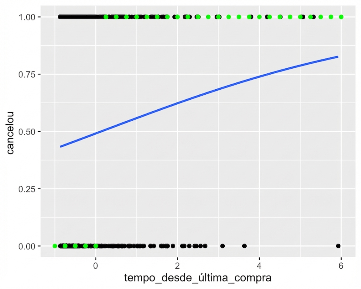
As previsões no ggplot

plt_churn_vs_recency_base <- ggplot(
  churn, 
  aes(time_since_last_purchase, has_churned)
) +
  geom_point() +
  geom_smooth(
    method = "glm", 
    se = FALSE, 
    method.args = list(family = binomial)
  )

Gráfico de dispersão de churn vs. tempo desde a última compra, com linha logística.

Fazendo previsões

mdl_recency <- glm(
  has_churned ~ time_since_last_purchase, data = churn, family = "binomial"
)

explanatory_data <- tibble(
  time_since_last_purchase = seq(-1, 6, 0.25)
)

prediction_data <- explanatory_data %>% 
  mutate(
    has_churned = predict(mdl_recency, explanatory_data, type = "response")
  )

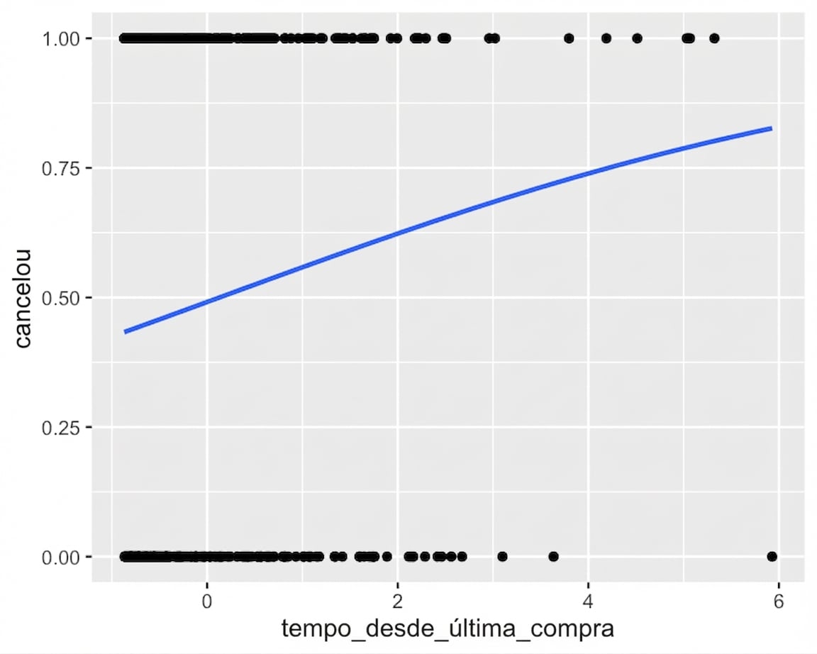
Adicionando previsões pontuais

plt_churn_vs_recency_base +
  geom_point(
    data = prediction_data, 
    color = "blue"
  )

Dispersão de churn vs. tempo desde a última compra, com linha logística. O gráfico é anotado com os resultados de predict(), que seguem exatamente a linha.

Obtendo o resultado mais provável

prediction_data <- explanatory_data %>% 
  mutate(
    has_churned = predict(mdl_recency, explanatory_data, type = "response"),
    most_likely_outcome = round(has_churned)
  )

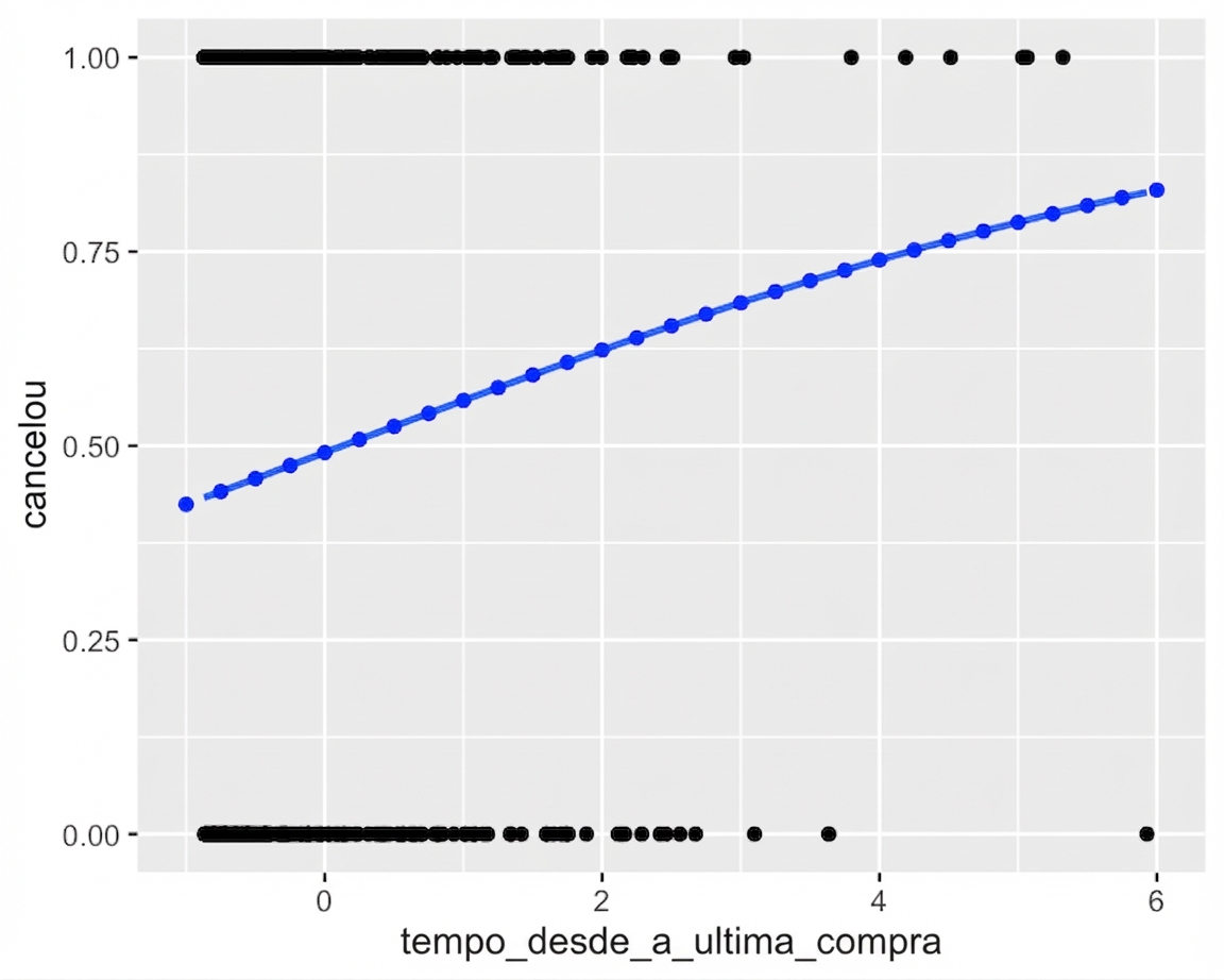
Visualizando o resultado mais provável

plt_churn_vs_recency_base +
  geom_point(
    aes(y = most_likely_outcome),
    data = prediction_data,
    color = "green"
  )

Dispersão de churn vs. tempo desde a última compra, com linha logística. O gráfico marca os resultados mais prováveis. Para baixo tempo desde a última compra, o mais provável é não churnar. Para alto tempo, o mais provável é churnar.

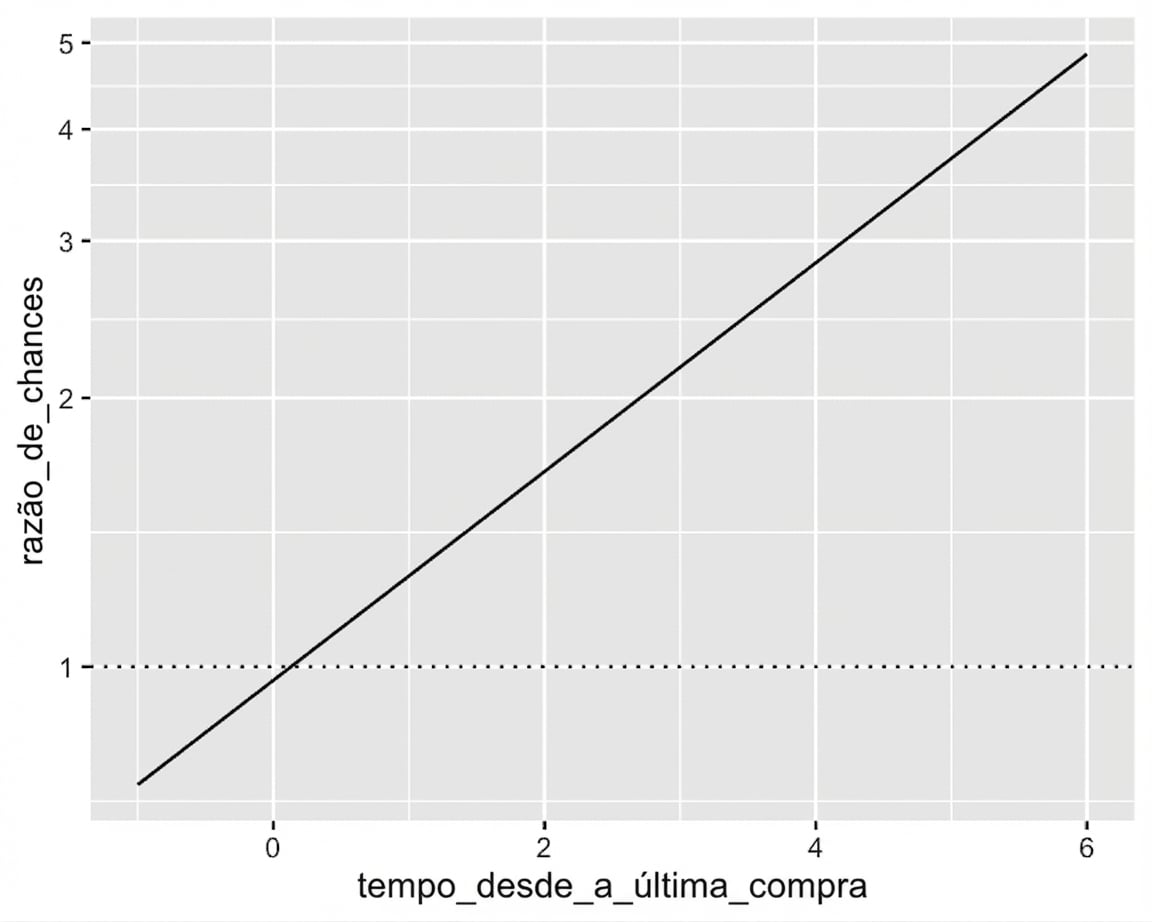
Razões de chance

A razão de chance é a probabilidade de algo acontecer dividida pela probabilidade de não acontecer.

$$ odds\_ratio = \frac{probability}{(1 - probability)} $$

$$ odds\_ratio = \frac{0.25}{(1 - 0.25)} = \frac{1}{3} $$

Gráfico de linha de razão de chance vs. probabilidade. A curva cresce assintoticamente ao infinito conforme a probabilidade tende a 1.

Calculando a razão de chance

prediction_data <- explanatory_data %>%
  mutate(
    has_churned = predict(mdl_recency, explanatory_data, type = "response"),
    most_likely_response = round(has_churned),
    odds_ratio = has_churned / (1 - has_churned)
  )

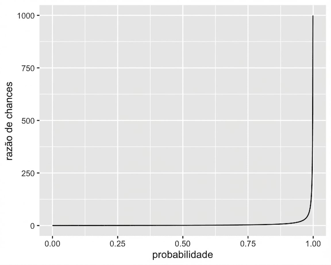
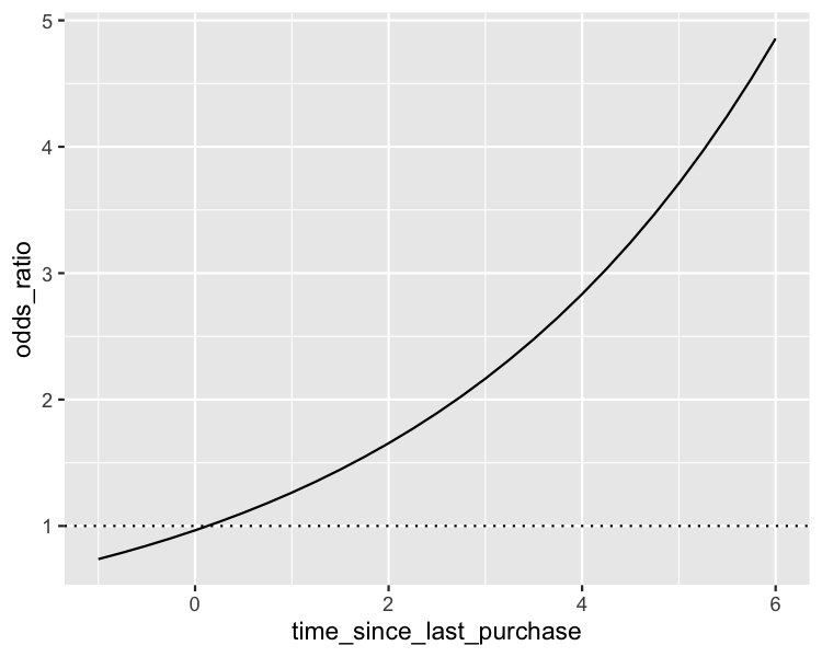
Visualizando a razão de chance

ggplot(
  prediction_data, 
  aes(time_since_last_purchase, odds_ratio)
) +
  geom_line() +
  geom_hline(yintercept = 1, linetype = "dotted")

Linha de razão de chance vs. tempo desde a última compra, com linha em razão de chance = 1. Para baixo tempo, o mais provável é não churnar. As chances de churn aumentam com o tempo, chegando a até cinco vezes as de não churnar.

Visualizando log da razão de chance

ggplot(
  prediction_data, 
  aes(time_since_last_purchase, odds_ratio)
) +
  geom_line() +
  geom_hline(yintercept = 1, linetype = "dotted") +
  scale_y_log10()

O gráfico de razão de chance vs. tempo desde a última compra, com linha em razão de chance = 1. O eixo y está em escala logarítmica, deixando a linha das chances aproximadamente linear.

Calculando o log da razão de chance

prediction_data <- explanatory_data %>%
  mutate(
    has_churned = predict(mdl_recency, explanatory_data, type = "response"),
    most_likely_response = round(has_churned),
    odds_ratio = has_churned / (1 - has_churned),
    log_odds_ratio = log(odds_ratio),
    log_odds_ratio2 = predict(mdl_recency, explanatory_data)
  )

Todas as previsões juntas

tm_snc_lst_prch	has_churned	most_lkly_rspns	odds_ratio	log_odds_ratio	log_odds_ratio2
0	0.491	0	0.966	-0.035	-0.035
2	0.623	1	1.654	0.503	0.503
4	0.739	1	2.834	1.042	1.042
6	0.829	1	4.856	1.580	1.580
...	...	...	...	...	...

Comparando escalas

Escala	Valores fáceis de interpretar?	Mudanças fáceis de interpretar?	É precisa?
Probabilidade	✔	✘	✔
Resultado mais provável	✔✔	✔	✘
Razão de chance	✔	✘	✔
Log da razão de chance	✘	✔	✔

Vamos praticar!

Introdução à Regressão em R