Conclusão
Análise Exploratória de Dados em R

Andrew Bray
Assistant Professor, Reed College
Gráfico de pizza vs. barras
Facetar vs. empilhar
Histograma
ggplot(data, aes(x = var1)) +
    geom_histogram()
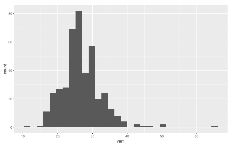
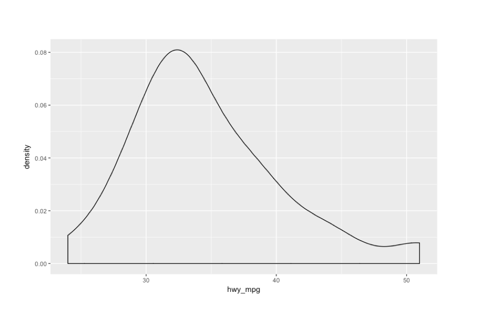
Gráfico de densidade
cars %>%
  filter(eng_size < 2.0) %>%
  ggplot(aes(x = hwy_mpg)) +
  geom_density()
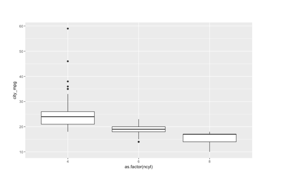
Boxplots lado a lado
ggplot(common_cyl, aes(x = as.factor(ncyl), y = city_mpg)) +
  geom_boxplot()
Warning message:
Removed 11 rows containing non-finite values (stat_boxplot).
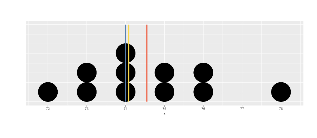
Centro: média, mediana, moda
x
76 78 75 74 76 72 74 73 73 75 74
table(x)
x
72 73 74 75 76 78
 1  2  3  2  2  1
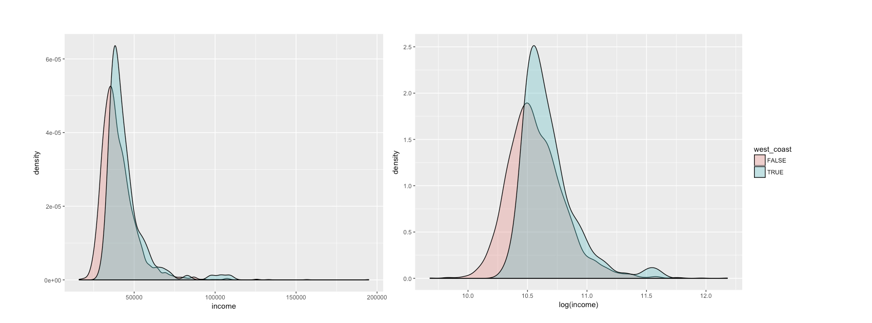
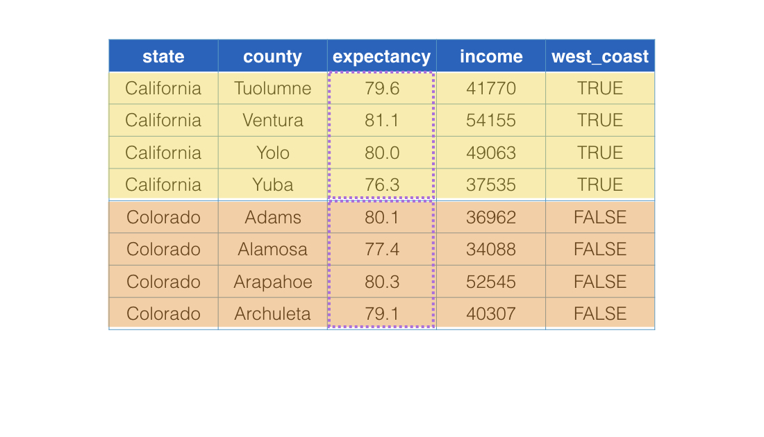
Distribuição da renda
ggplot(life, aes(x = income, fill = west_coast)) +
  geom_density(alpha = .3)
ggplot(life, aes(x = log(income), fill = west_coast)) +
  geom_density(alpha = .3)
Com group_by()
life %>%
  slice(240:247) %>%
  group_by(west_coast) %>%
  summarize(mean(expectancy))
# A tibble: 2 x 2
  west_coast mean(expectancy)
       <lgl           <dbl>
1      FALSE         79.26125
2       TRUE         79.29375
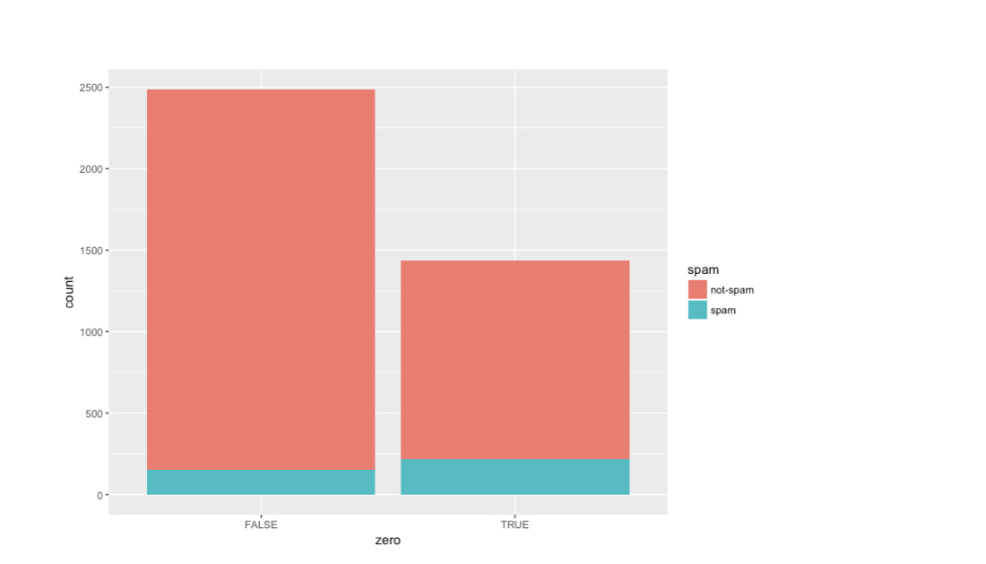
Spam e pontos de exclamação
email %>%
  mutate(zero = exclaim_mess == 0) %>%
  ggplot(aes(x = zero, fill = spam)) +
  geom_bar()
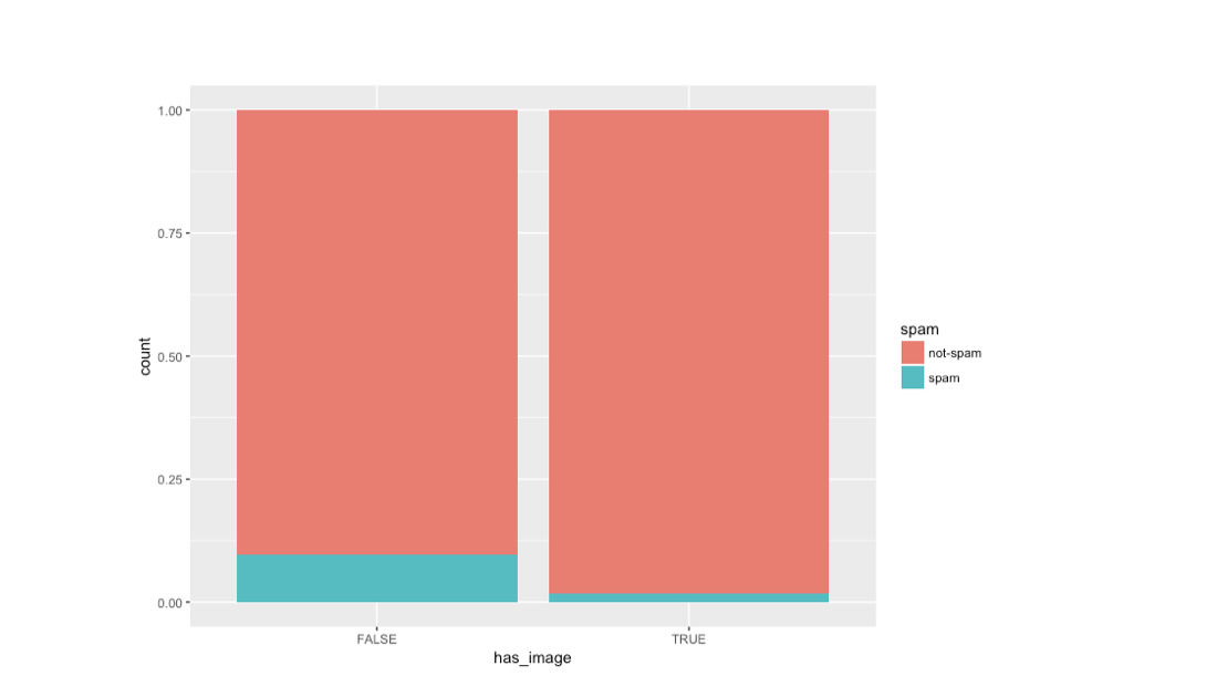
Spam e imagens
email %>%
  mutate(has_image = image 0) %>%
  ggplot(aes(x = as.factor(has_image), fill = spam)) +
  geom_bar(position = "fill")