Medidas de centro
Análise Exploratória de Dados em R

Andrew Bray
Assistant Professor, Reed College
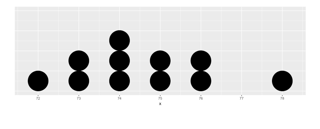
Centro: média
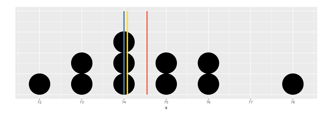
x <- head(round(life$expectancy), 11)
x
76 78 75 74 76 72 74 73 73 75 74
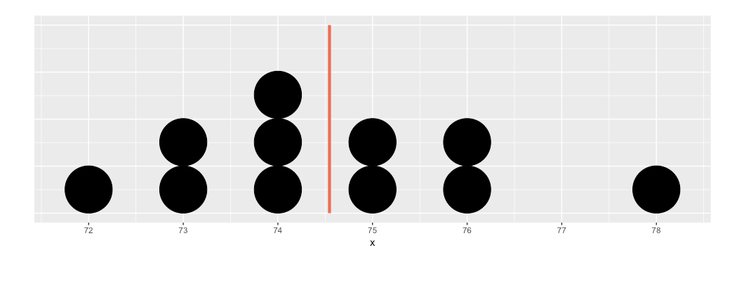
Centro: média
sum(x)/11
74.54545
mean(x)
74.54545
Centro: média
sum(x)/11
74.54545
mean(x)
74.54545
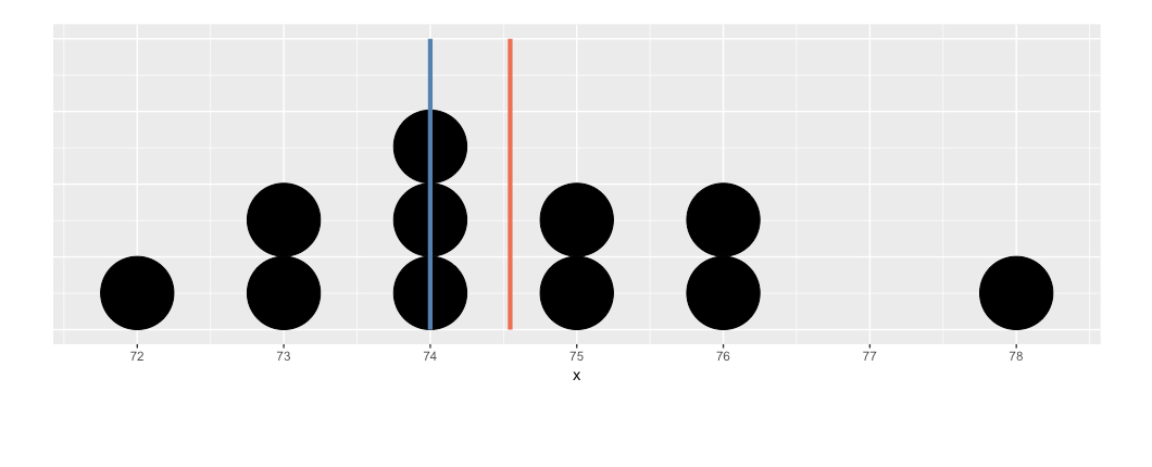
Centro: média, mediana
sort(x)
72 73 73 74 74 74 75 75 76 76 78
median(x)
74

Centro: média, mediana
sort(x)
72 73 73 74 74 74 75 75 76 76 78
median(x)
74

Centro: média, mediana, moda
table(x)
x
72 73 74 75 76 78
 1  2  3  2  2  1
Centro: média, mediana, moda
table(x)
x
72 73 74 75 76 78
 1  2  3  2  2  1
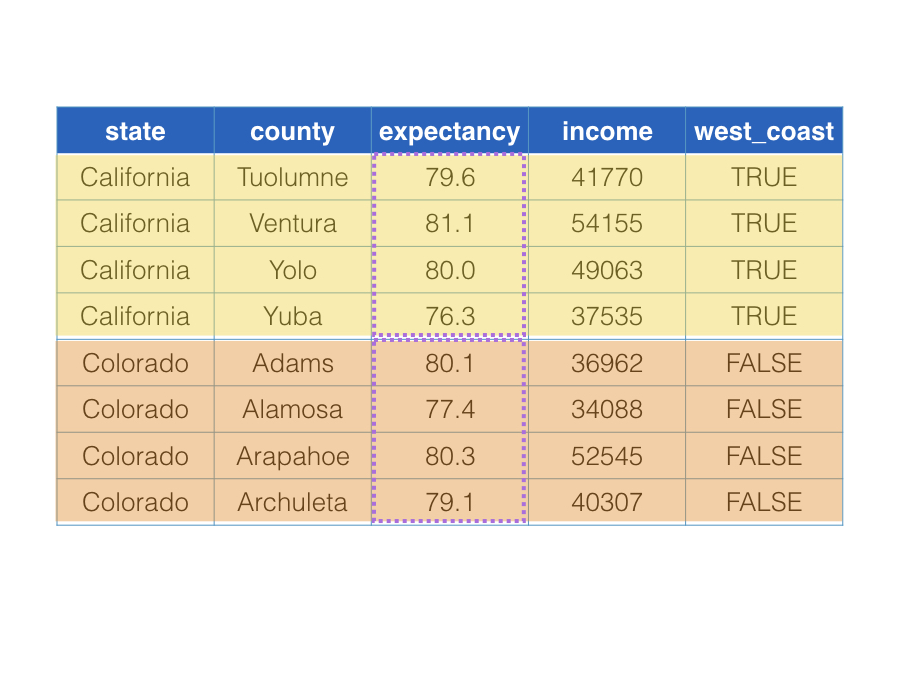
Sem group_by()
life %>%
  slice(240:247) %>%
  summarize(mean(expectancy))
# A tibble: 1 x 1
  mean(expectancy)
             <dbl>
1          79.2775
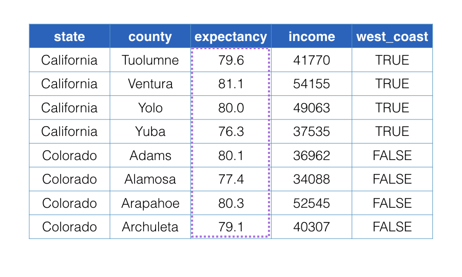
Com group_by()
life %>%
  slice(240:247) %>%
  group_by(west_coast) %>%
  summarize(mean(expectancy))
# A tibble: 2 x 2
  west_coast mean(expectancy)
       <lgl           <dbl>
1      FALSE         79.26125
2       TRUE         79.29375