Transformando variáveis

Introdução à Regressão com statsmodels em Python

Maarten Van den Broeck

Content Developer at DataCamp

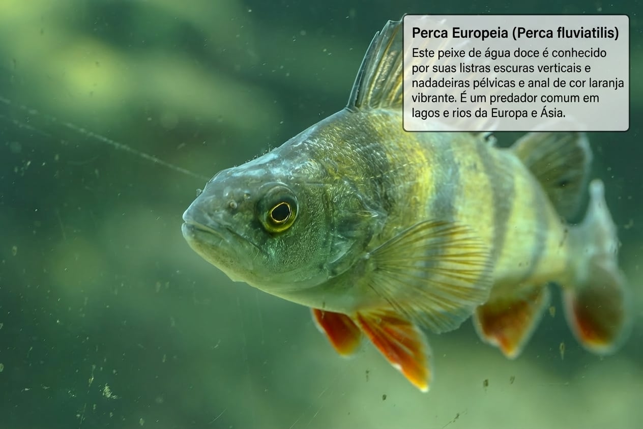
Conjunto de dados de perca

perch = fish[fish["species"] == "Perch"]
print(perch.head())

   species  mass_g  length_cm
55   Perch     5.9        7.5
56   Perch    32.0       12.5
57   Perch    40.0       13.8
58   Perch    51.5       15.0
59   Perch    70.0       15.7

Perca europeia, _Perca fluviatilis_

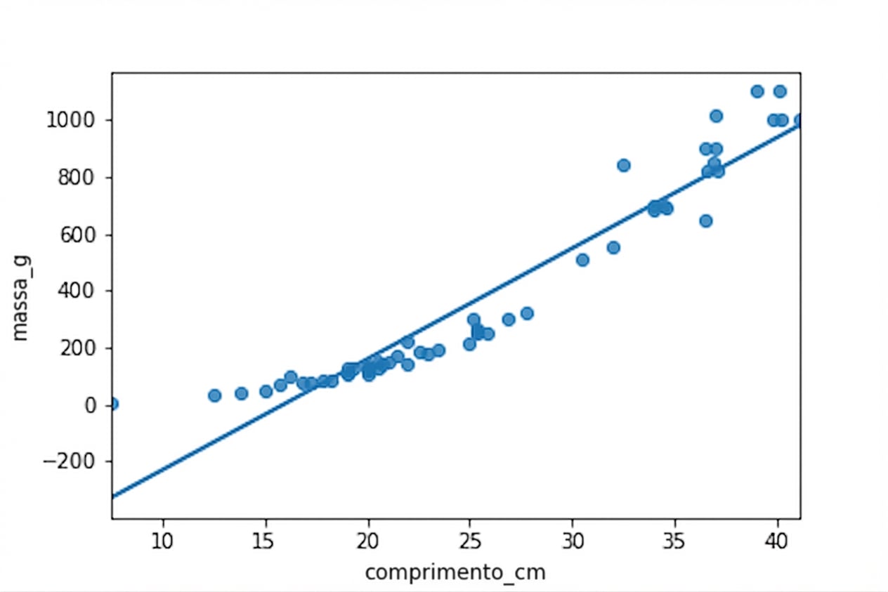
Não é uma relação linear

sns.regplot(x="length_cm",
            y="mass_g",
            data=perch,
            ci=None)

plt.show()

Um gráfico de dispersão das massas de perca versus seus comprimentos, com uma linha de tendência. As percas ficam mais pesadas mais rápido do que linearmente à medida que crescem, resultando em uma curva ascendente.

Brema vs. perca

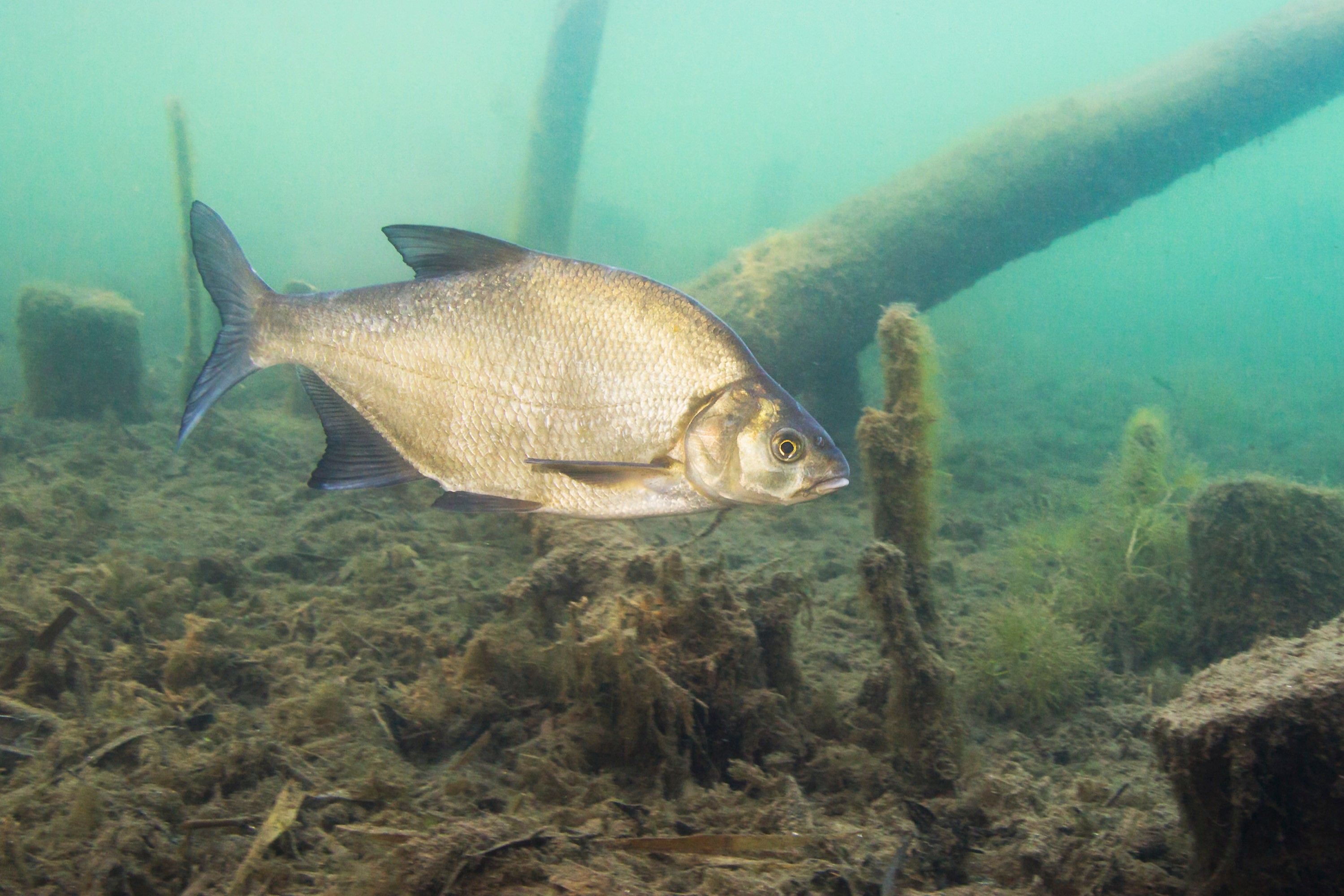
Um brema comum. Bremas são bastante achatadas.

Uma perca europeia. Perca são bastante arredondadas.

Gráfico: massa vs. comprimento³

perch["length_cm_cubed"] = perch["length_cm"] ** 3

sns.regplot(x="length_cm_cubed",
            y="mass_g",
            data=perch,
            ci=None)
plt.show()

Um gráfico de dispersão das massas de perca versus seus comprimentos ao cubo, com uma linha de tendência. Após essa transformação, os pontos estão próximos da linha de tendência.

Modelando massa vs. comprimento³

perch["length_cm_cubed"] = perch["length_cm"] ** 3

mdl_perch = ols("mass_g ~ length_cm_cubed", data=perch).fit()
mdl_perch.params

Intercept         -0.117478
length_cm_cubed    0.016796
dtype: float64

Prevendo massa vs. comprimento³

explanatory_data = pd.DataFrame({"length_cm_cubed": np.arange(10, 41, 5) ** 3,
                                 "length_cm": np.arange(10, 41, 5)})

prediction_data = explanatory_data.assign(
  mass_g=mdl_perch.predict(explanatory_data))
print(prediction_data)

   length_cm_cubed  length_cm       mass_g
0             1000         10    16.678135
1             3375         15    56.567717
2             8000         20   134.247429
3            15625         25   262.313982
4            27000         30   453.364084
5            42875         35   719.994447
6            64000         40  1074.801781

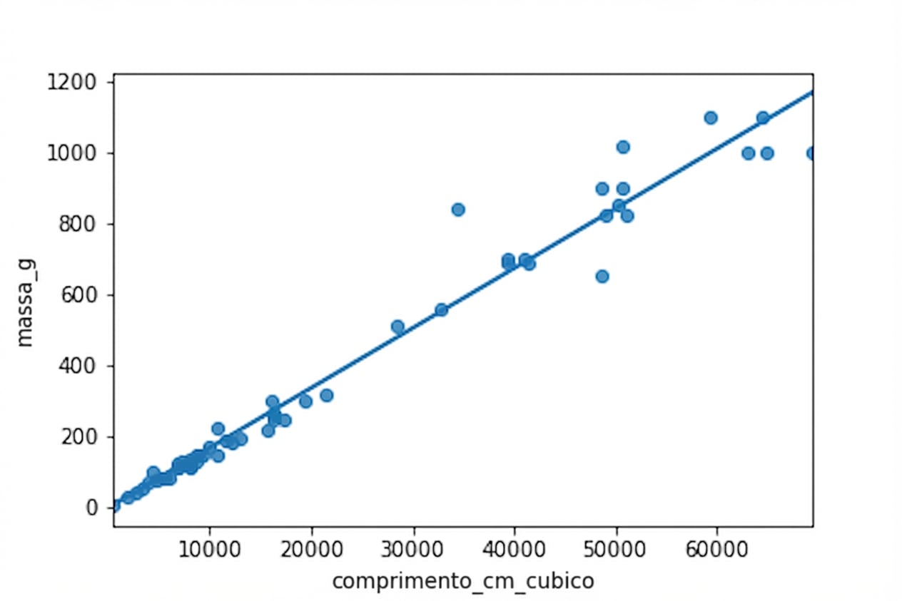
Gráfico: massa vs. comprimento³

fig = plt.figure()
sns.regplot(x="length_cm_cubed", y="mass_g",
            data=perch, ci=None)
sns.scatterplot(data=prediction_data,
                x="length_cm_cubed", y="mass_g",
                color="red", marker="s")

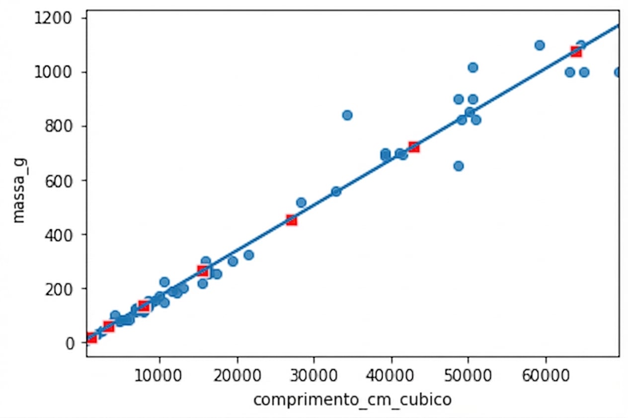
O gráfico de dispersão das massas de perca versus seus comprimentos ao cubo, com uma linha de tendência, anotado com pontos calculados a partir da função predict(). Os pontos seguem exatamente a linha de tendência.

fig = plt.figure()
sns.regplot(x="length_cm", y="mass_g",
            data=perch, ci=None)
sns.scatterplot(data=prediction_data,
                x="length_cm", y="mass_g",
                color="red", marker="s")

O gráfico de dispersão das massas de perca versus seus comprimentos, com uma linha de tendência, anotado com pontos calculados a partir da função predict(). Os pontos não seguem a linha de tendência, mas seguem a curva dos pontos de dados.

Conjunto de dados de anúncios do Facebook

Como funciona a publicidade

Pague ao Facebook para mostrar anúncios.
Pessoas veem os anúncios ("impressões").
Algumas pessoas clicam.

936 linhas
Cada linha representa 1 anúncio

spent_usd	n_impressions	n_clicks
1.43	7350	1
1.82	17861	2
1.25	4259	1
1.29	4133	1
4.77	15615	3
...	...	...

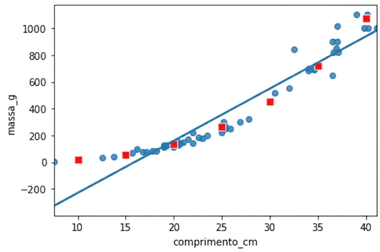
Gráfico está apertado

sns.regplot(x="spent_usd",
            y="n_impressions",
            data=ad_conversion,
            ci=None)

Um gráfico de dispersão do número de impressões versus o gasto com publicidade, com uma linha de tendência. A maioria dos pontos de dados está concentrada no canto inferior esquerdo do gráfico.

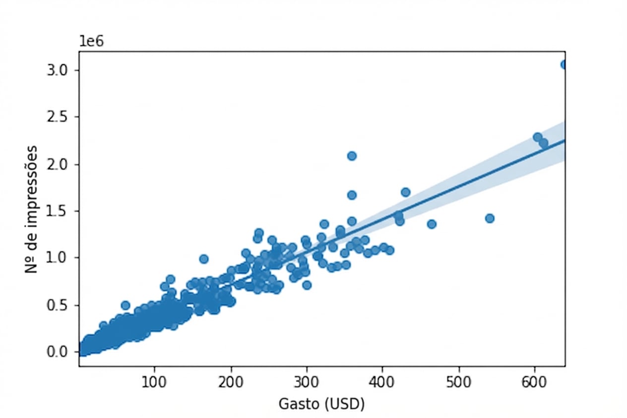
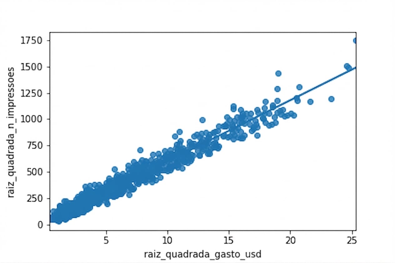
Raiz quadrada vs raiz quadrada

ad_conversion["sqrt_spent_usd"] = np.sqrt(
  ad_conversion["spent_usd"])

ad_conversion["sqrt_n_impressions"] = np.sqrt(
  ad_conversion["n_impressions"])

sns.regplot(x="sqrt_spent_usd",
            y="sqrt_n_impressions",
            data=ad_conversion,
            ci=None)

Um gráfico de dispersão da raiz quadrada do número de impressões versus a raiz quadrada do gasto com publicidade, com uma linha de tendência. Agora os pontos estão mais distribuídos pelo gráfico.

Modelando e prevendo

mdl_ad = ols("sqrt_n_impressions ~ sqrt_spent_usd", data=ad_conversion).fit()

explanatory_data = pd.DataFrame({"sqrt_spent_usd": np.sqrt(np.arange(0, 601, 100)),
                                 "spent_usd": np.arange(0, 601, 100)})

prediction_data = explanatory_data.assign(sqrt_n_impressions=mdl_ad.predict(explanatory_data),
                          n_impressions=mdl_ad.predict(explanatory_data) ** 2)
print(prediction_data)

   sqrt_spent_usd  spent_usd  sqrt_n_impressions  n_impressions
0        0.000000          0           15.319713   2.346936e+02
1       10.000000        100          597.736582   3.572890e+05
2       14.142136        200          838.981547   7.038900e+05
3       17.320508        300         1024.095320   1.048771e+06
4       20.000000        400         1180.153450   1.392762e+06
5       22.360680        500         1317.643422   1.736184e+06
6       24.494897        600         1441.943858   2.079202e+06

Vamos praticar!

Introdução à Regressão com statsmodels em Python