Visualizando o ajuste do modelo
Introdução à Regressão com statsmodels em Python

Maarten Van den Broeck
Content Developer at DataCamp
Tainha e perca novamente
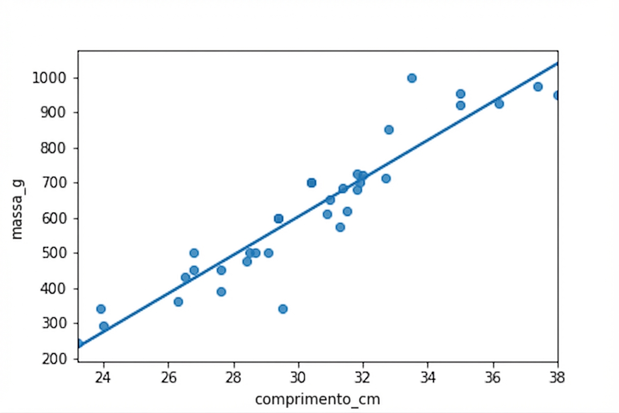
Tainha: o modelo "bom"
mdl_bream = ols("mass_g ~ length_cm", data=bream).fit()
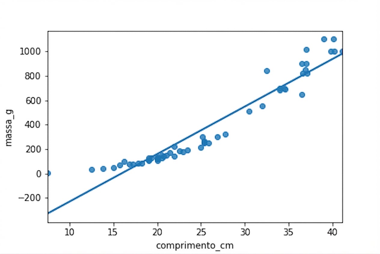
Perca: o modelo "ruim"
mdl_perch = ols("mass_g ~ length_cm", data=perch).fit()
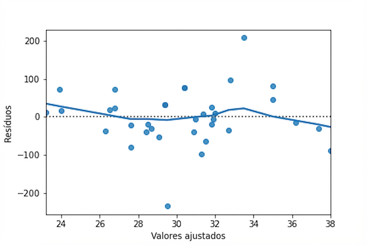
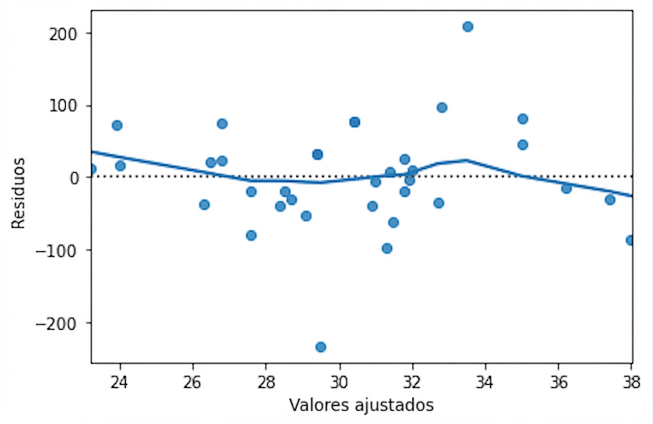
Resíduos vs. ajustados
Tainha
Perca
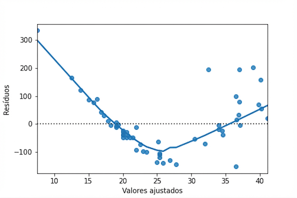
Gráfico Q-Q
Tainha
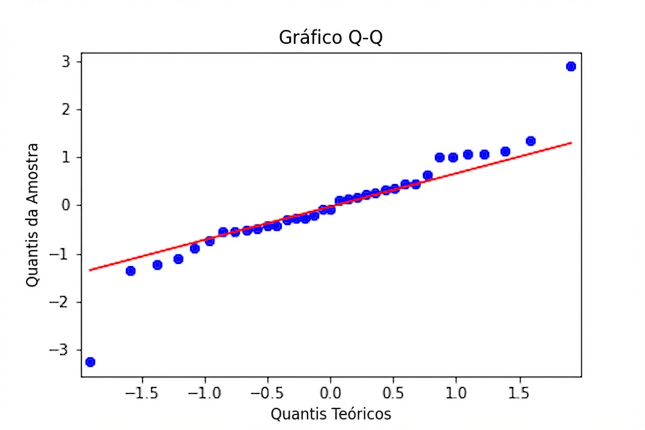
Perca
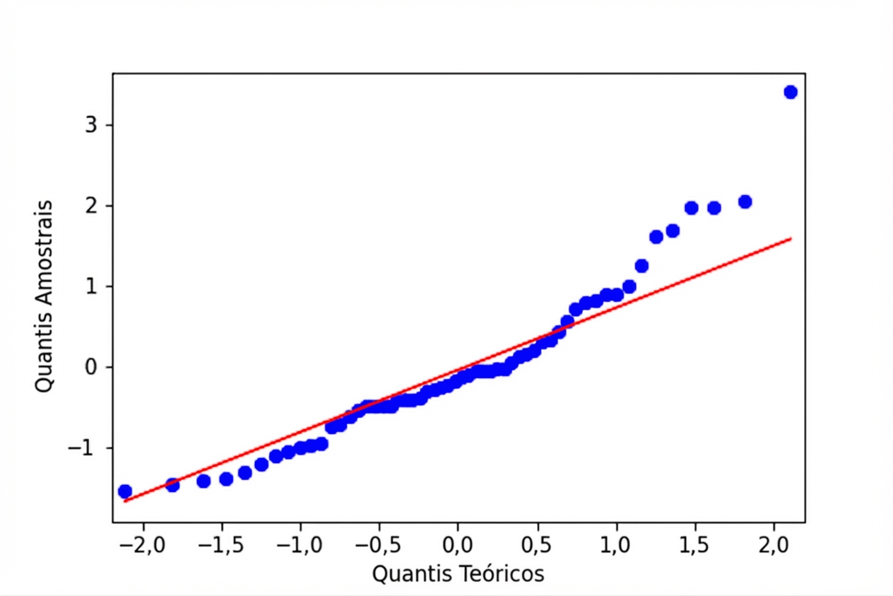
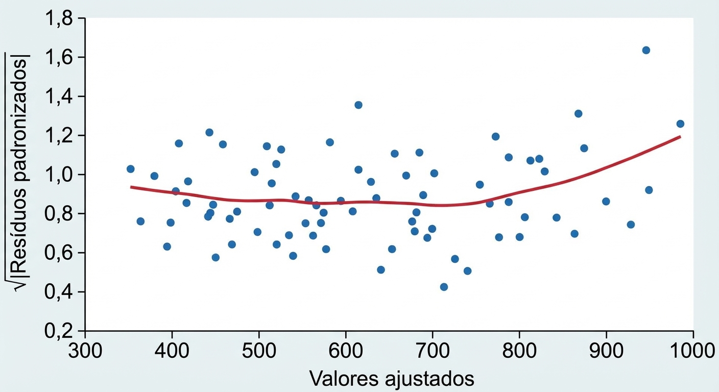
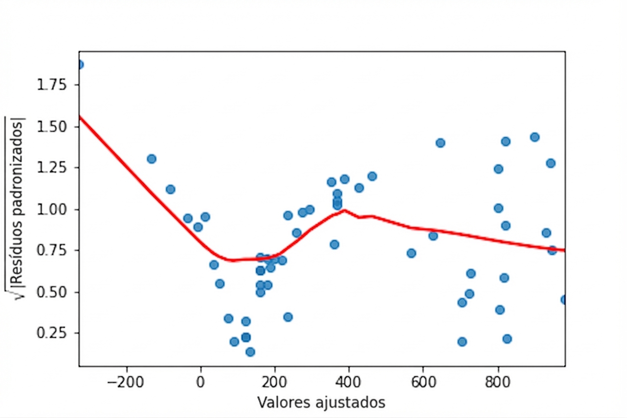
Gráfico de escala-localização
Tainha
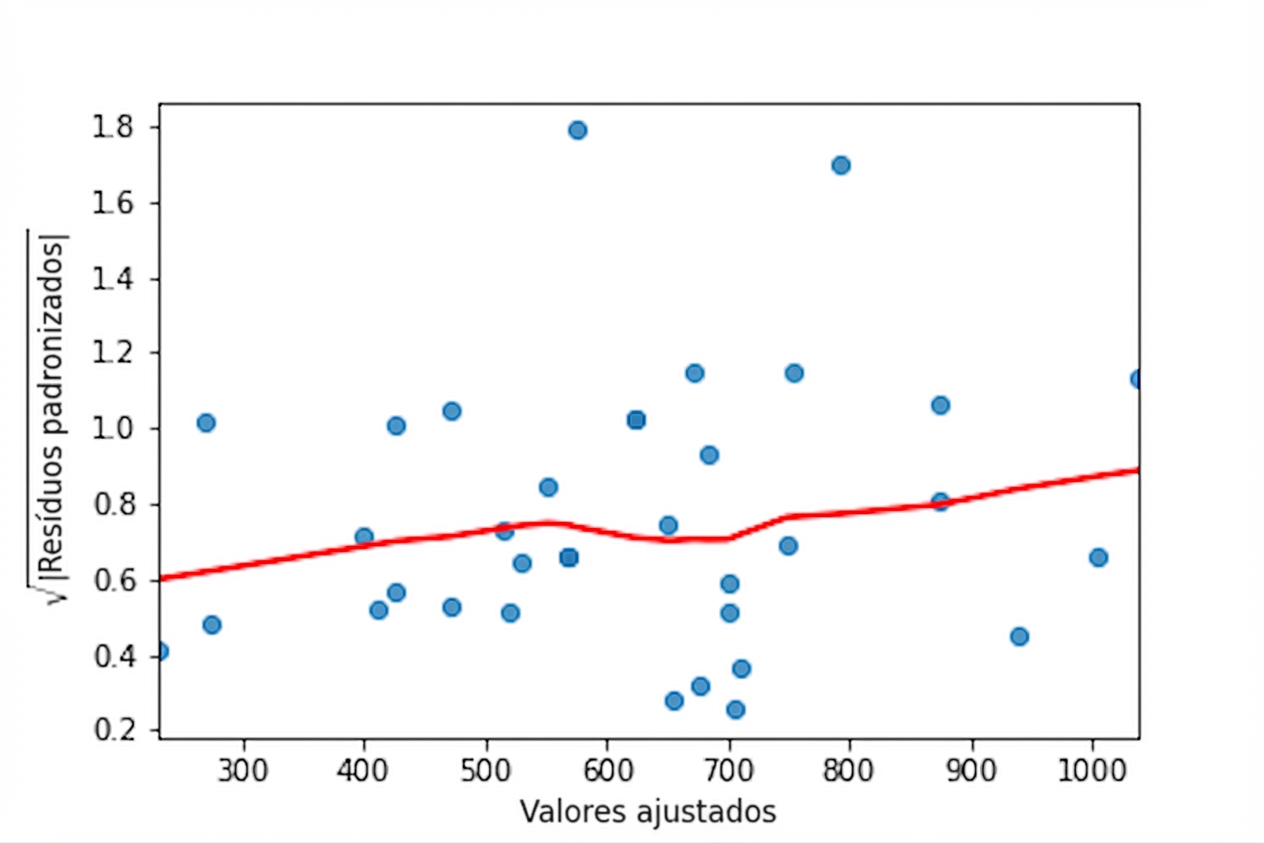
Perca
residplot()
sns.residplot(x="length_cm", y="mass_g", data=bream, lowess=True)
plt.xlabel("Valores ajustados")
plt.ylabel("Resíduos")
qqplot()
from statsmodels.api import qqplot
qqplot(data=mdl_bream.resid, fit=True, line="45")
Gráfico de escala-localização
model_norm_residuals_bream = mdl_bream.get_influence().resid_studentized_internalmodel_norm_residuals_abs_sqrt_bream = np.sqrt(np.abs(model_norm_residuals_bream))sns.regplot(x=mdl_bream.fittedvalues, y=model_norm_residuals_abs_sqrt_bream, ci=None, lowess=True)plt.xlabel("Valores ajustados") plt.ylabel("Raiz do valor abs dos resíduos padronizados")