Ampliando funções de janela com pandas
Manipulando dados de séries temporais em Python

Stefan Jansen
Founder & Lead Data Scientist at Applied Artificial Intelligence
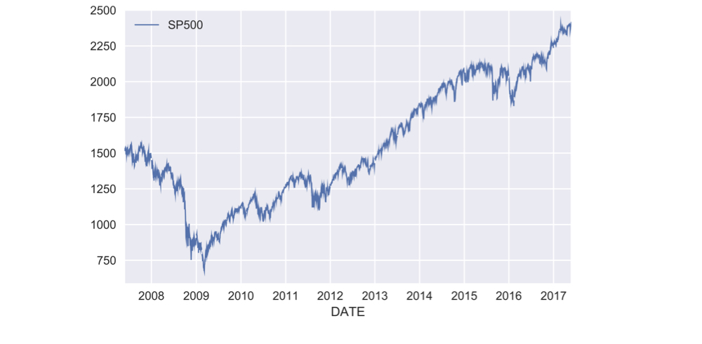
Obtenha dados do S&P 500
data = pd.read_csv('sp500.csv', parse_dates=['date'], index_col='date')
DatetimeIndex: 2519 entries, 2007-05-24 to 2017-05-24
Data columns (total 1 columns):
SP500    2519 non-null float64
Retorno acumulado na prática
pr = data.SP500.pct_change() # period returnpr_plus_one = pr.add(1)cumulative_return = pr_plus_one.cumprod().sub(1)cumulative_return.mul(100).plot()

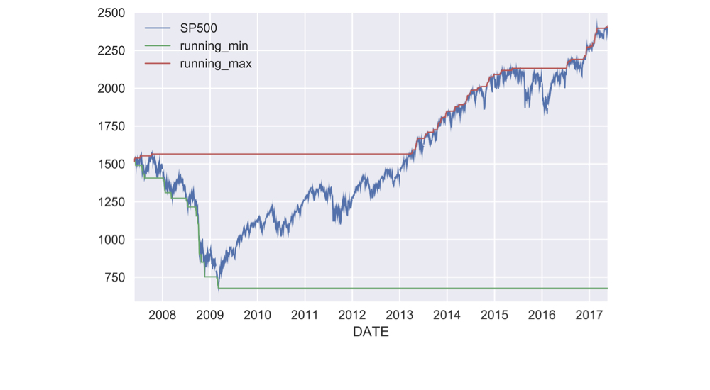
Obtendo o min e max correntes
data['running_min'] = data.SP500.expanding().min()data['running_max'] = data.SP500.expanding().max()data.plot()
Retorno anual móvel
data['Rolling 1yr Return'] = r.mul(100)data.plot(subplots=True)


