Liniendiagramme

Einführung in die Datenvisualisierung mit ggplot2

Rick Scavetta

Founder, Scavetta Academy

Gängige Diagrammtypen

Diagrammtyp	Mögliche Geome
Streudiagramme	points, jitter, abline, smooth, count
Balkendiagramme	histogram, bar, col, errorbar
Liniendiagramme	line, path

Biber

str(beaver)

'data.frame':    101 obs. of  3 variables:
 $ time  : POSIXct, format: "2000-01-01 09:30:00" "2000-01-01 09:40:00" "2000-01-01 09:50:00" ...
 $ temp  : num  36.6 36.7 36.9 37.1 37.2 ...
 $ active: Factor w/ 2 levels "0","1": 1 1 1 1 1 1 1 1 1 1 ...

Biber

ggplot(beaver, aes(x = time, y = temp)) +
  geom_line()

Biber

ggplot(beaver, aes(x = time, y = temp, 
                   color = factor(active))
                   ) +
  geom_line()

Der Fischfang-Datensatz

str(fish)

'data.frame':    427 obs. of  3 variables:
 $ Species: Factor w/ 7 levels "Pink","Chum",..: 1 2 3 4 5 6 7 1 2 3 ...
 $ Year   : int  1950 1950 1950 1950 1950 1950 1950 1951 1951 1951 ...
 $ Capture: int  100600 139300 64100 30500 0 23200 10800 259000 155900 51200 ...

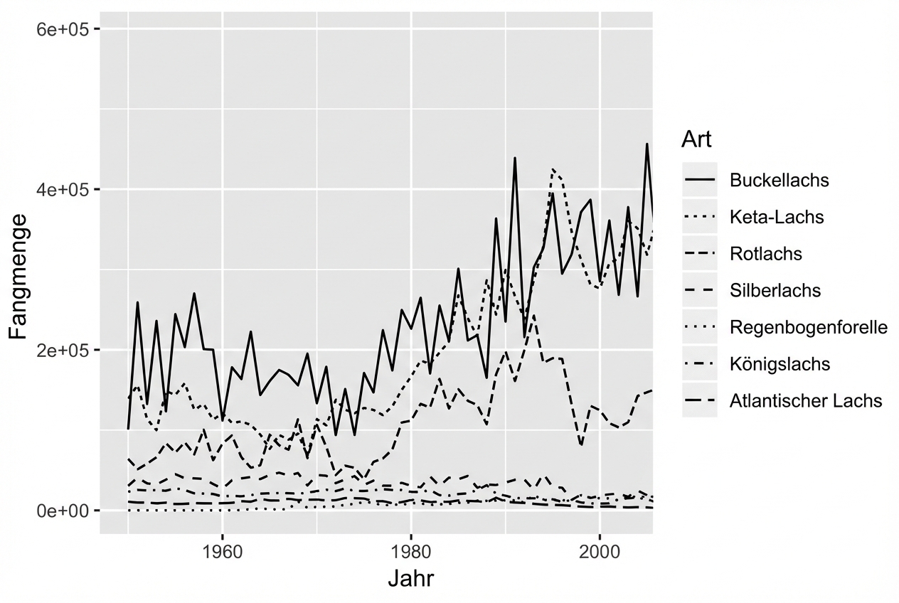
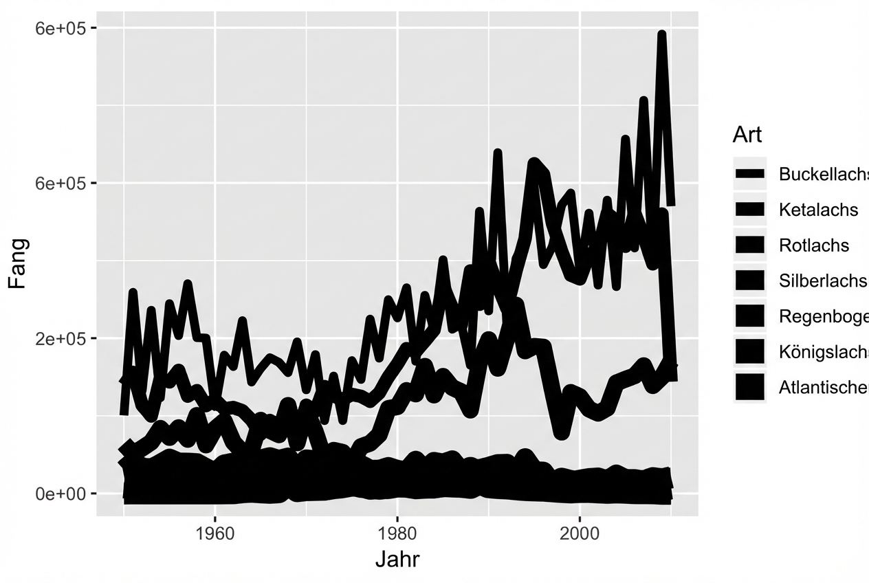
Ästhetisches Element Linientyp (linetype)

ggplot(fish, aes(x = Year, 
                 y = Capture, 
                 linetype = Species)) + 
  geom_line()

Ästhetisches Element Größe (size)

ggplot(fish, aes(x = Year, 
                 y = Capture, 
                 size = Species)) + 
  geom_line()

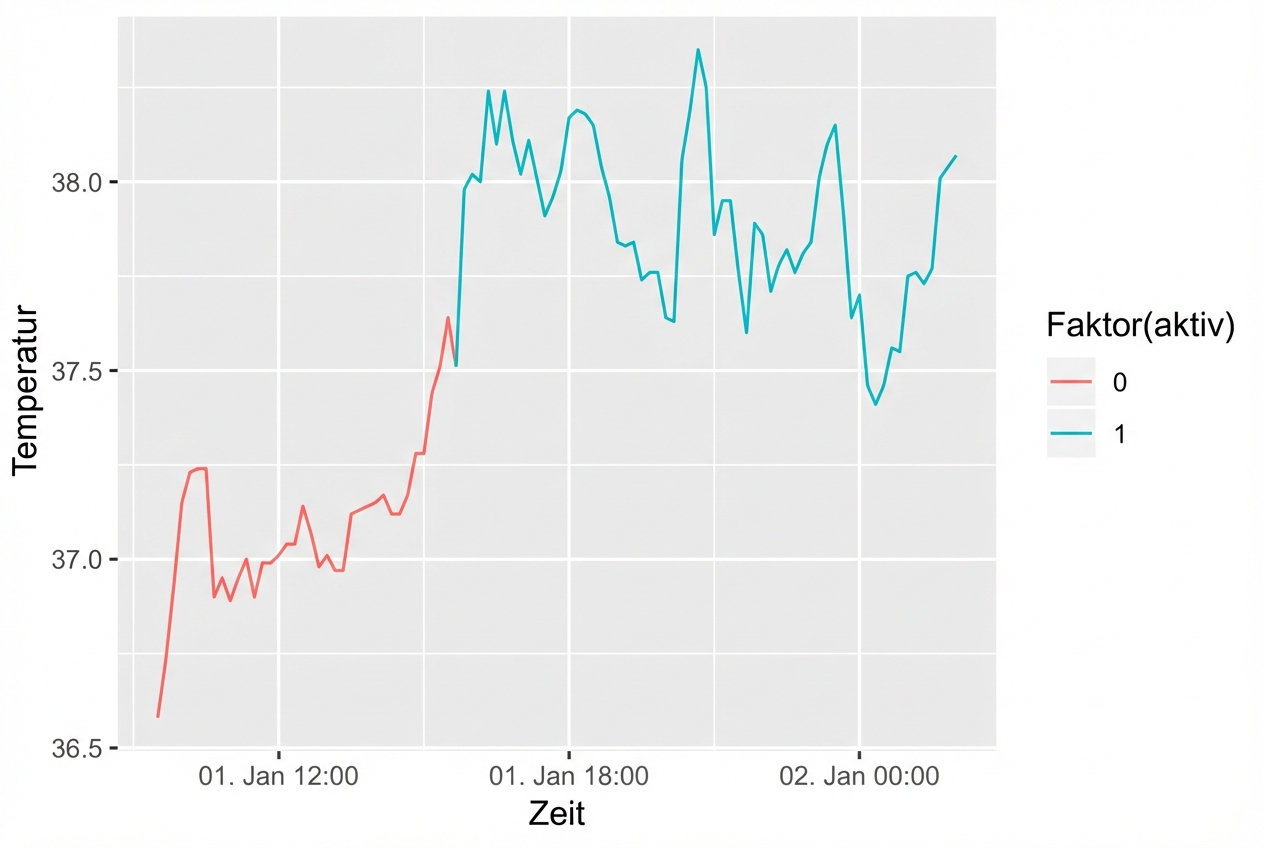
Ästhetische Element Farbe (color)

ggplot(fish, aes(x = Year, 
                 y = Capture, 
                 color = Species)) + 
  geom_line()

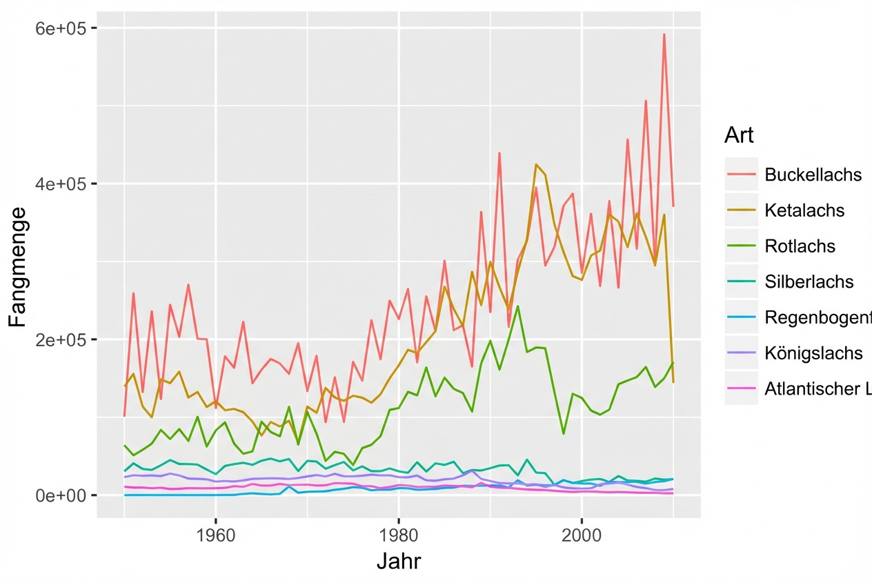
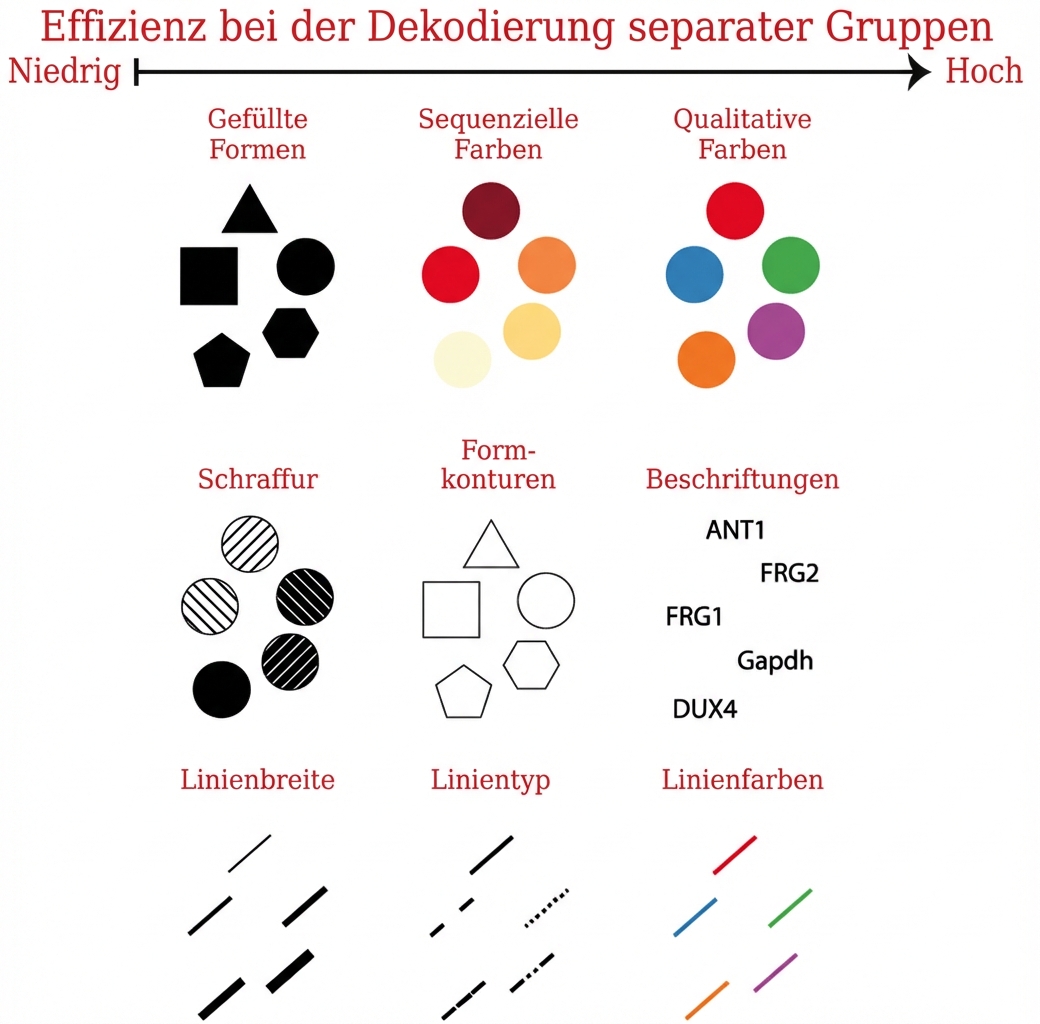
Ästhetische Elemente für kategoriale Variablen

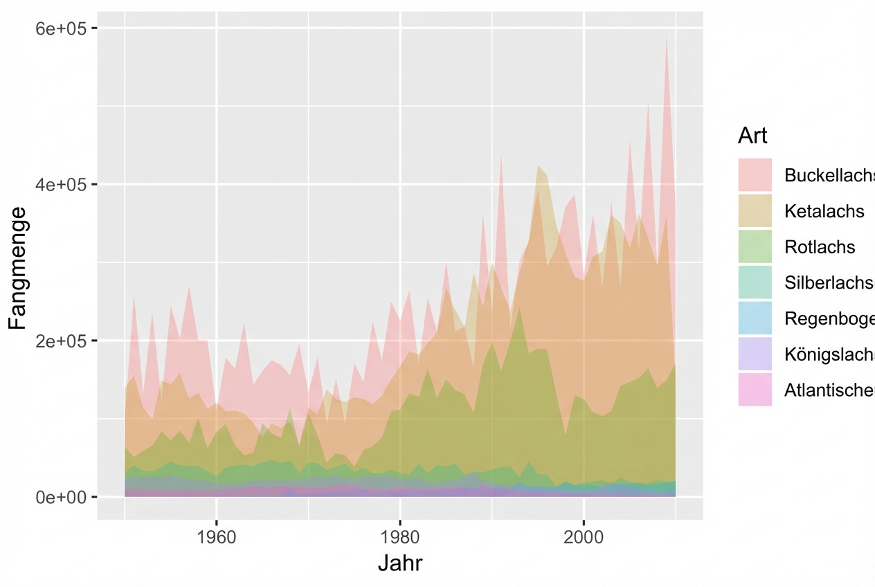
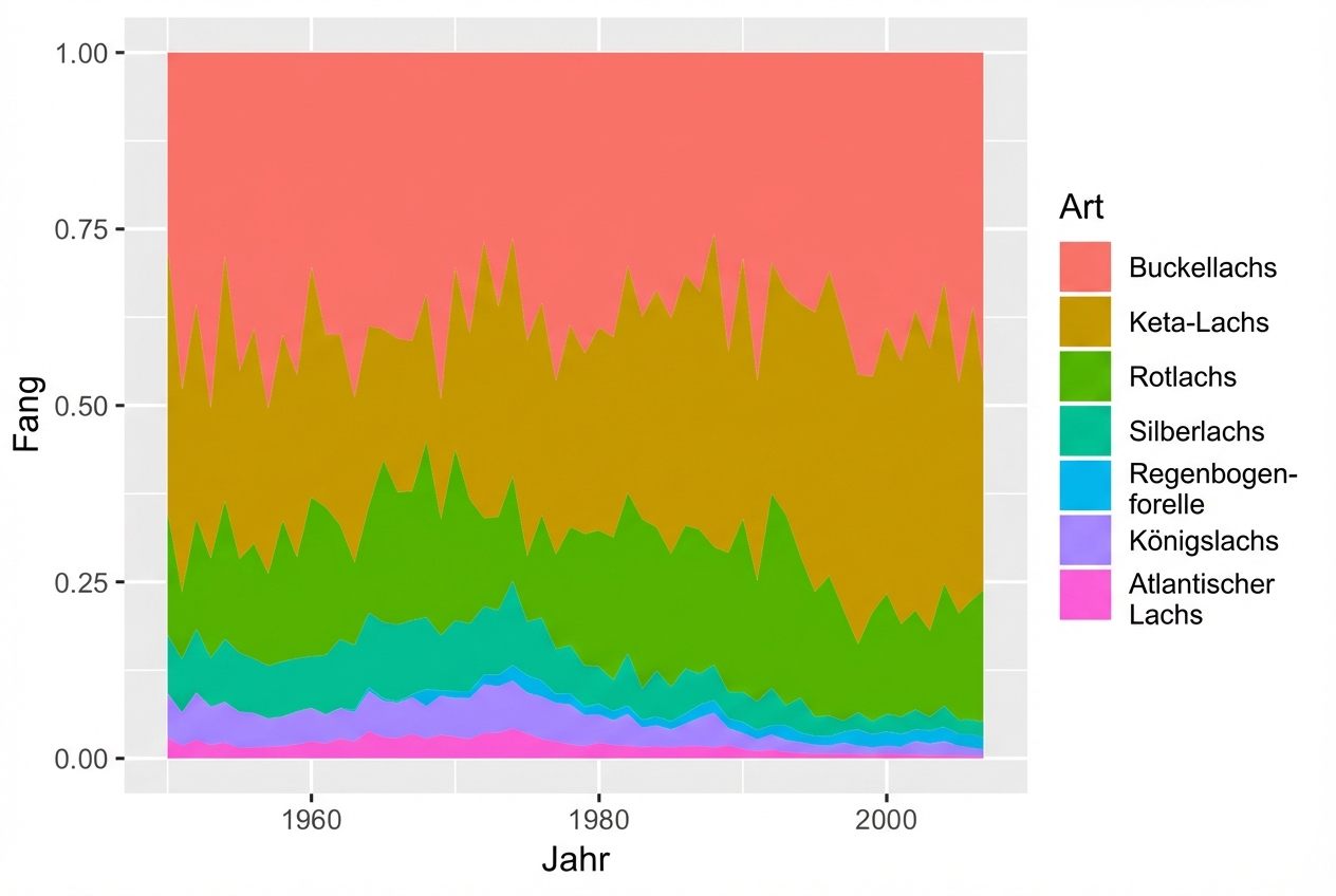
Ästhetisches Element Füllung (fill) mit geom_area()

ggplot(fish, aes(x = Year, 
                 y = Capture, 
                 fill = Species)) + 
  geom_area()

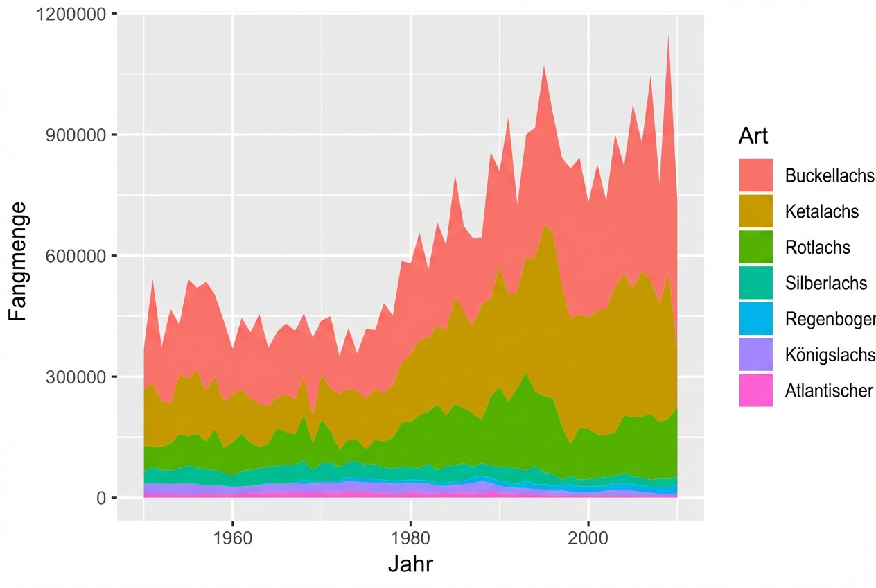
Mit position = "fill"

ggplot(fish, aes(x = Year, 
                 y = Capture, 
                 fill = Species)) + 
  geom_area(position = "fill")

geom_ribbon()

ggplot(fish, aes(x = Year, 
                 y = Capture, 
                 fill = Species)) + 
  geom_ribbon(aes(ymax = Capture, 
                  ymin = 0), 
              alpha = 0.3)

Lass uns üben!

Einführung in die Datenvisualisierung mit ggplot2