Ändern der ästhetischen Elemente
Einführung in die Datenvisualisierung mit ggplot2

Rick Scavetta
Founder, Scavetta Academy
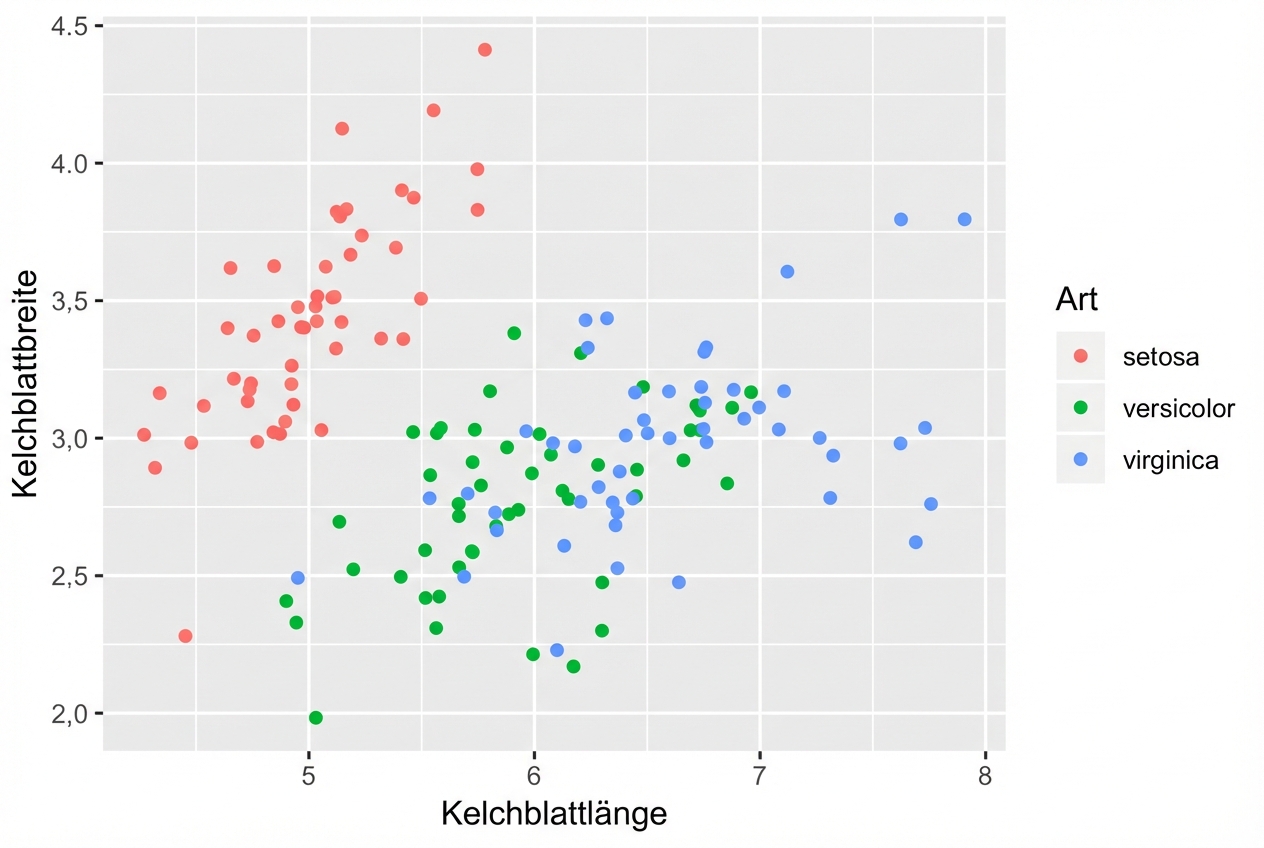
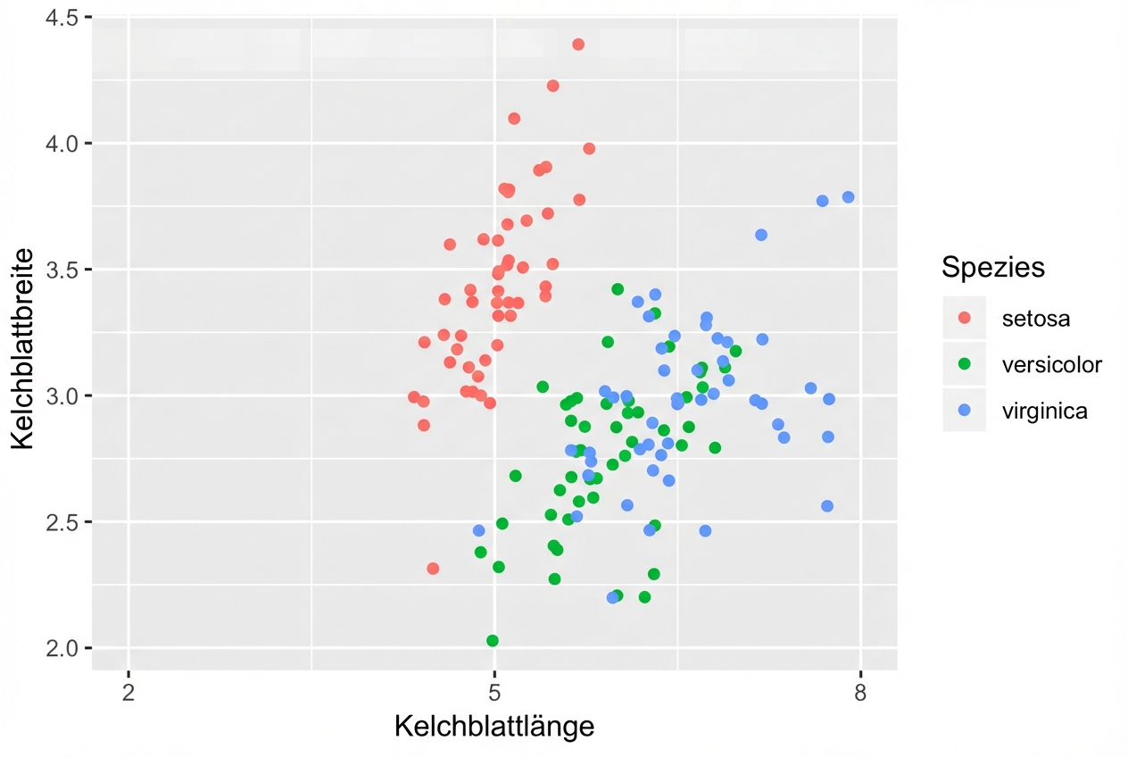
Position = "identity" (Standard)
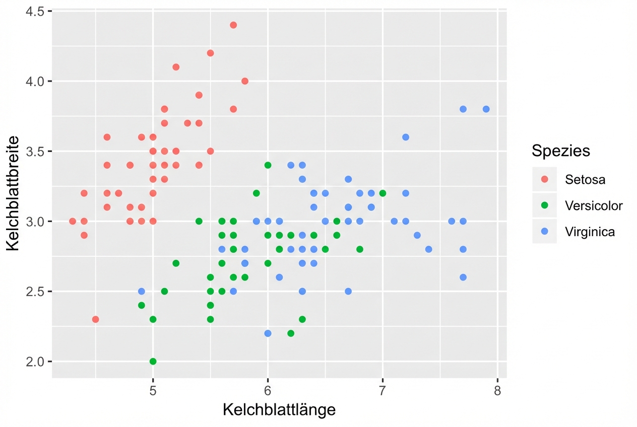
Position = "identity" (Standard)
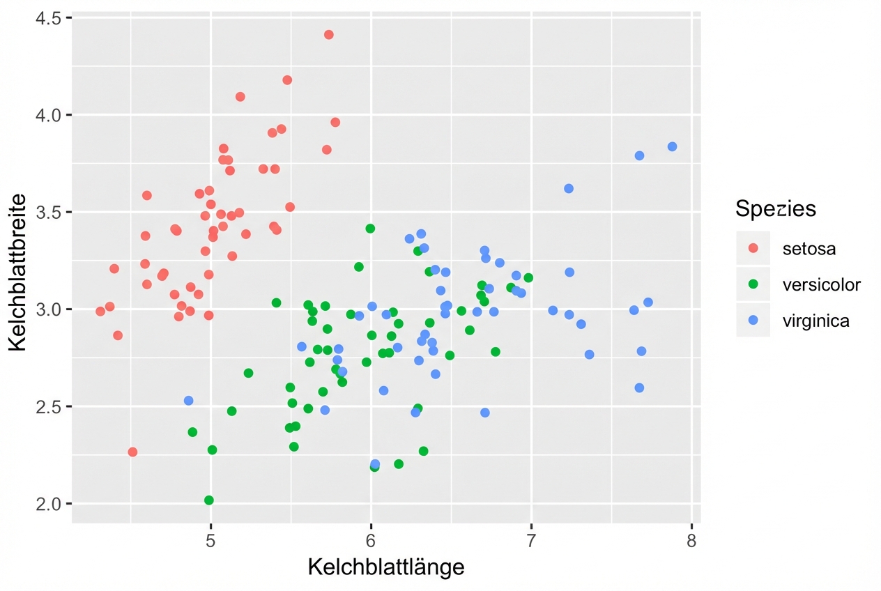
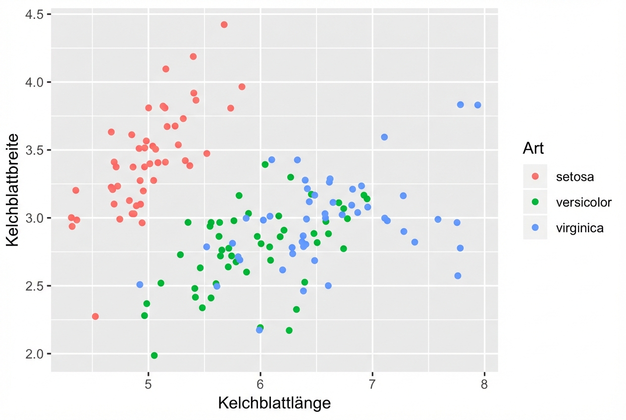
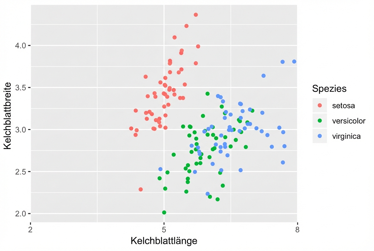
position = "jitter"
position_jitter()
position_jitter()
scale_*_*()
Das limits-Argument
Das breaks-Argument
Das expand-Argument
Das labels-Argument
labs()