Vorbehalte bei der Korrelation
Einführung in die Statistik in Python

Maggie Matsui
Content Developer, DataCamp
Nicht-lineare Beziehungen
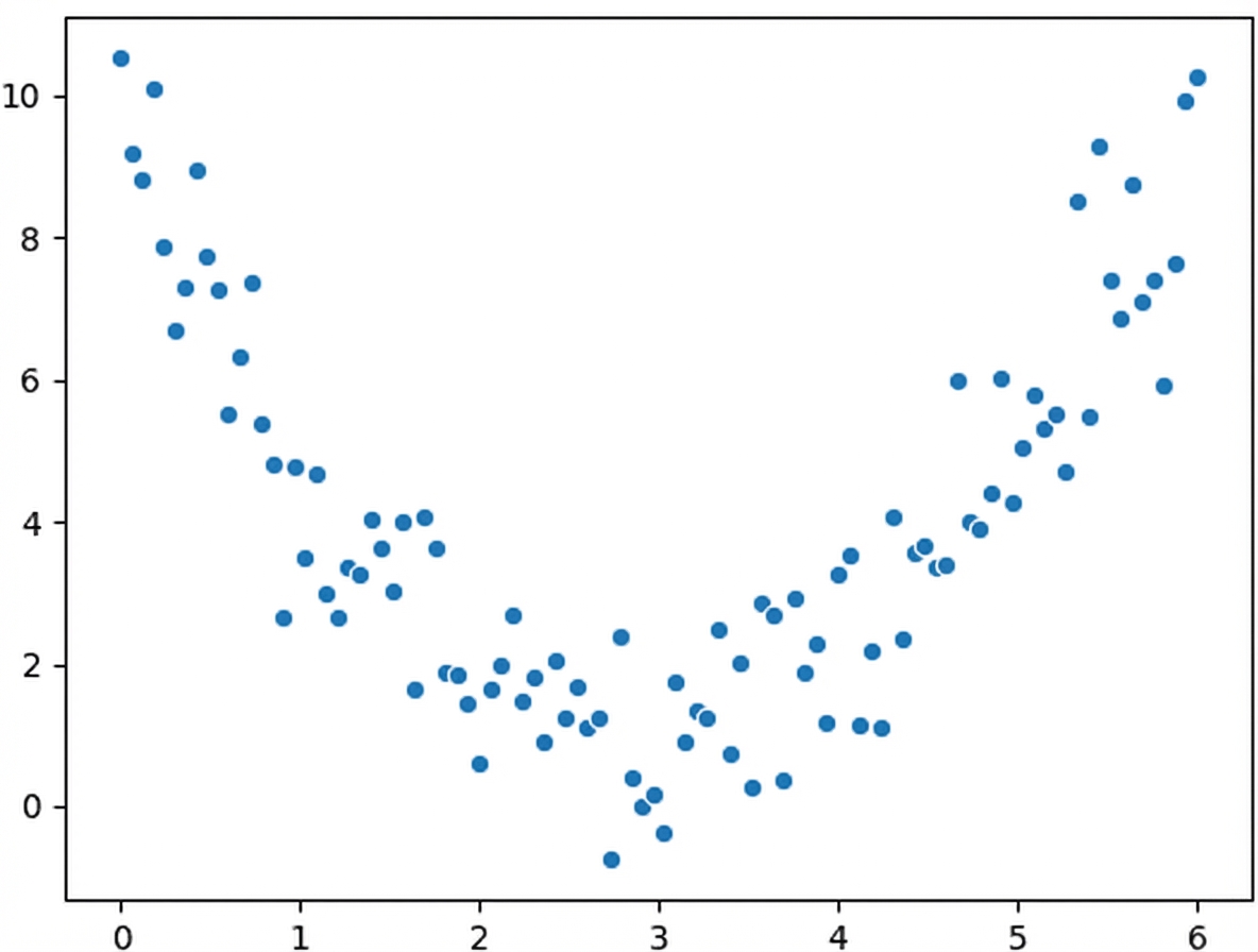
$$r = 0.18$$
Nicht-lineare Beziehungen
Was wir sehen:
Was der Korrelationskoeffizient sieht:
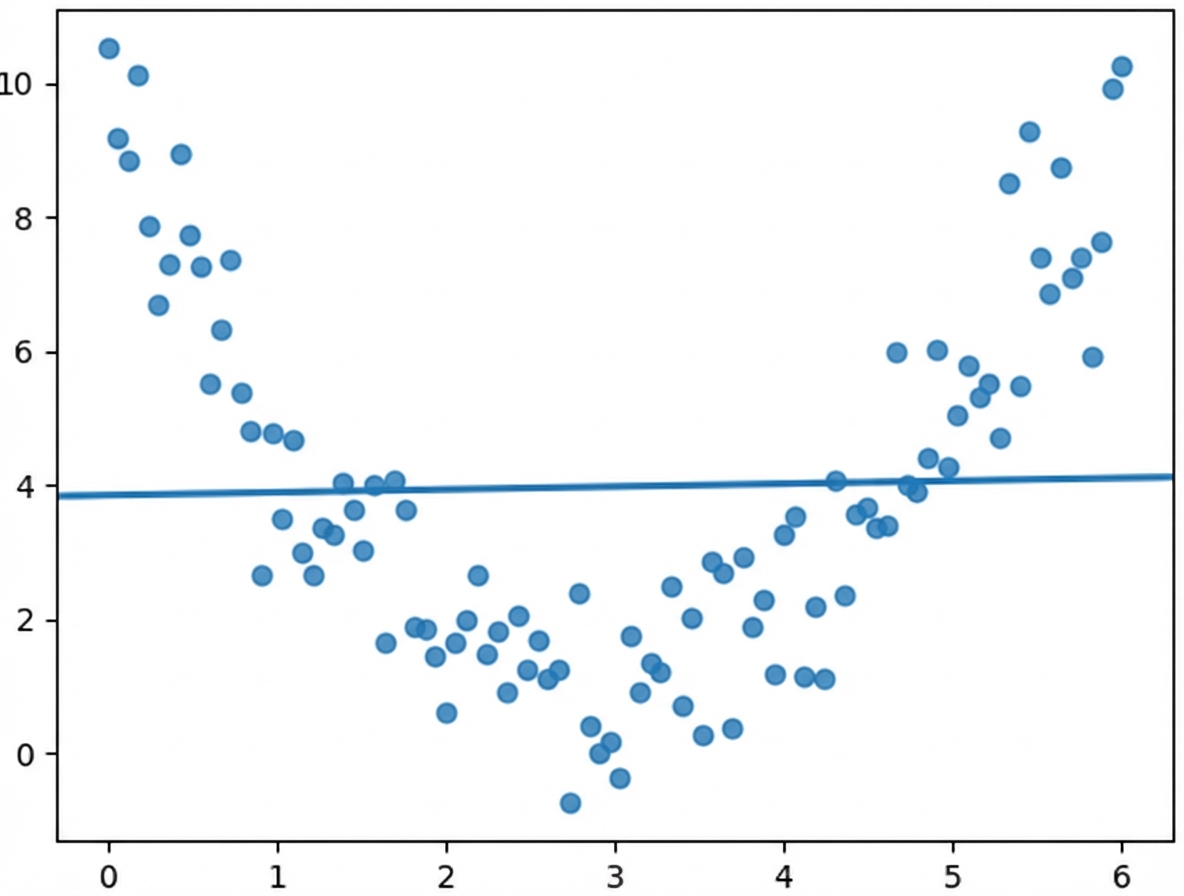
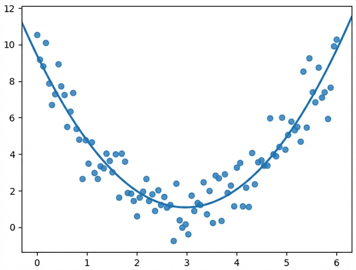
Die Korrelation berücksichtigt nur lineare Beziehungen
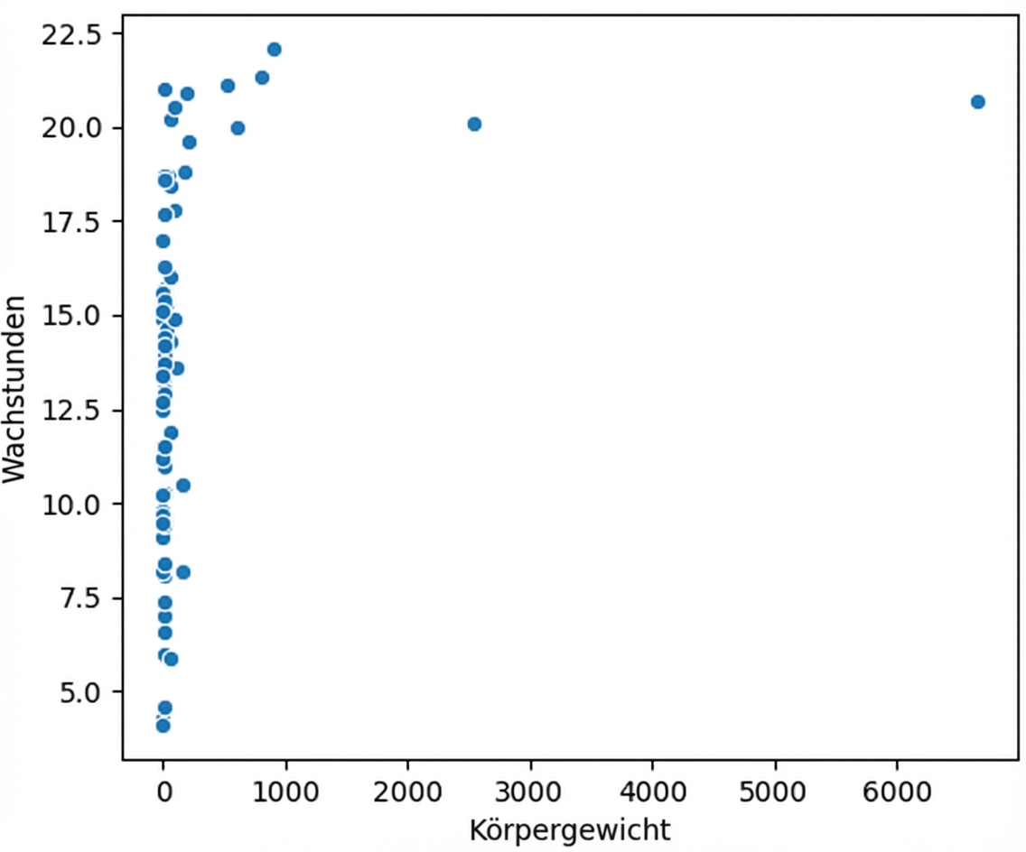
Visualisiere deine Daten immer
Körpergewicht vs. Wachzeit
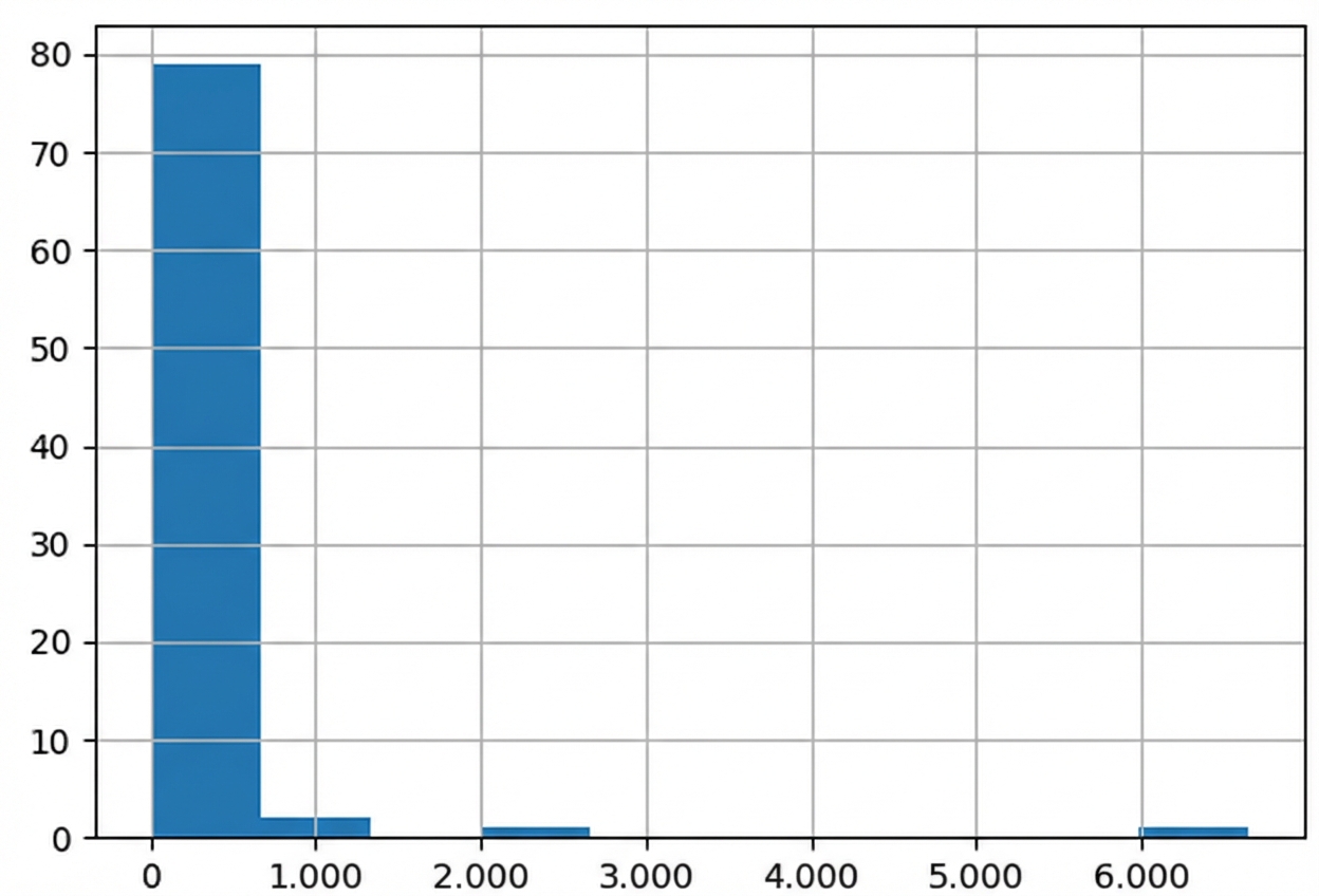
Verteilung des Körpergewichts
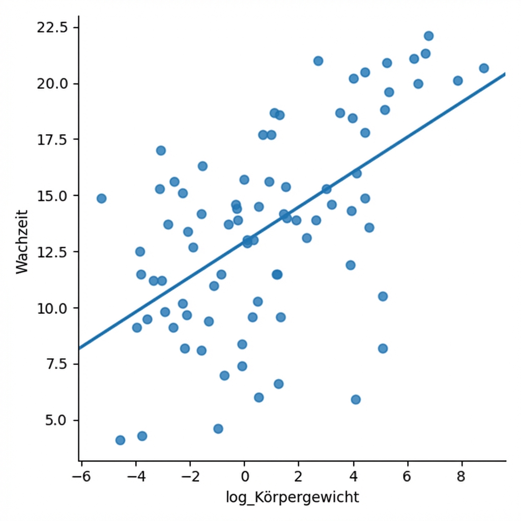
Log-Transformation
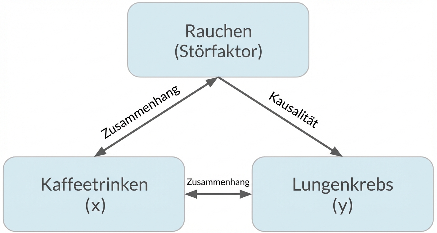
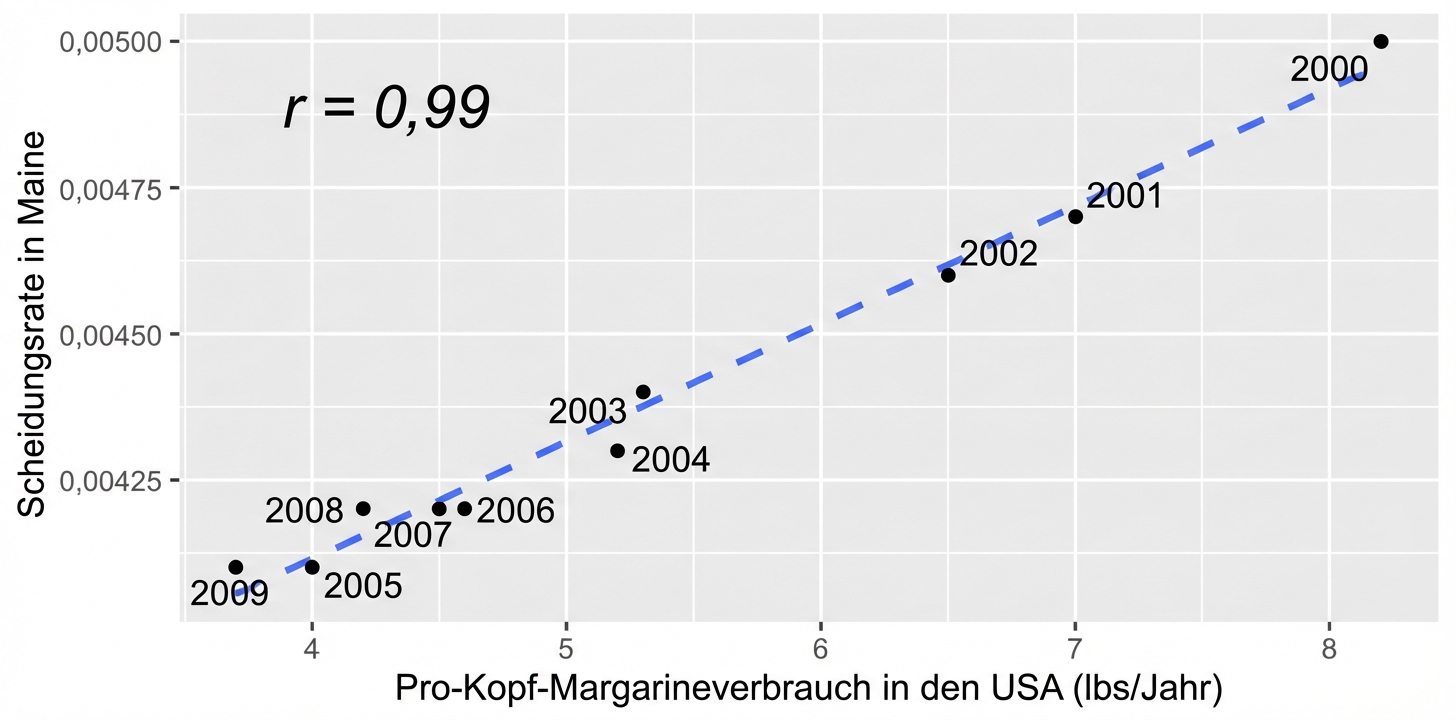
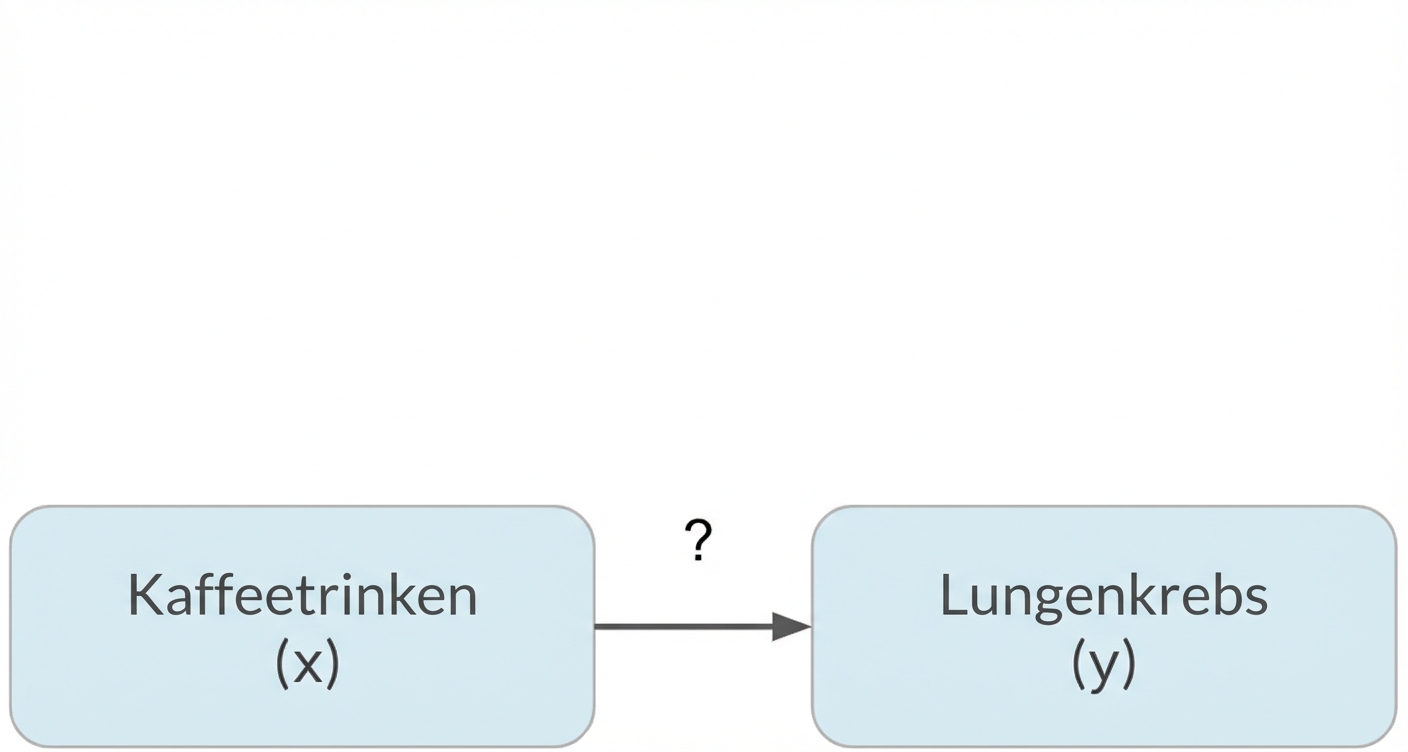
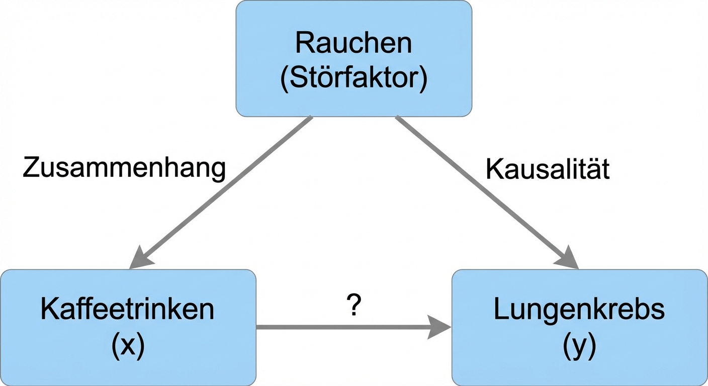
Korrelation bedeutet nicht gleich Kausalität
Wennx mit ykorreliert, bedeutet das nicht, dass x yverursacht
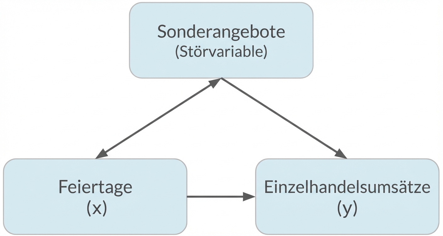
Verzerrungen
Verzerrungen
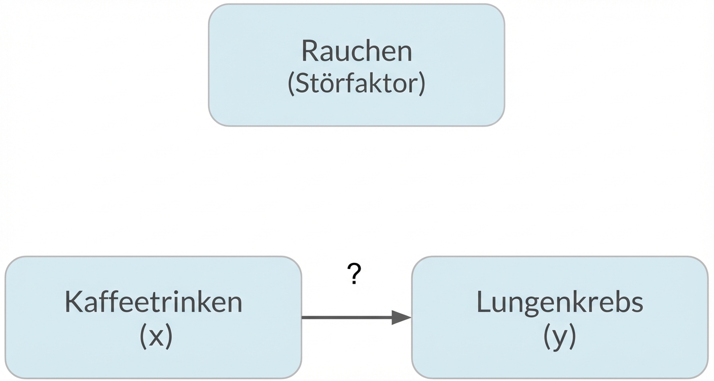
Verzerrungen
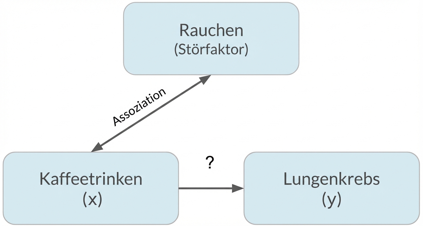
Verzerrungen
Verzerrungen