Maße der zentralen Tendenz

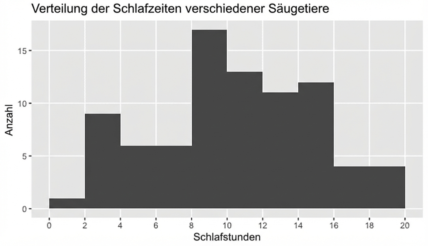
Einführung in die Statistik in R

Maggie Matsui

Content Developer, DataCamp

Daten zum Schlaf von Säugetieren

msleep

# A tibble: 83 x 11
   name             genus       vore  order        sleep_total sleep_rem sleep_cycle awake
   <chr>            <chr>       <chr> <chr>              <dbl>     <dbl>       <dbl> <dbl>
 1 Cheetah          Acinonyx    carni Carnivora           12.1      NA         NA     11.9
 2 Owl monkey       Aotus       omni  Primates            17         1.8       NA      7 
 3 Mountain beaver  Aplodontia  herbi Rodentia            14.4       2.4       NA      9.6
 4 Greater short... Blarina     omni  Soricomorpha        14.9       2.3       0.133   9.1 
 5 Cow              Bos         herbi Artiodactyla         4         0.7       0.667  20  
 6 Three-toed sloth Bradypus    herbi Pilosa              14.4       2.2       0.767   9.6 
 7 Northern fur...  Callorhinus carni Carnivora            8.7       1.4       0.383  15.3 
# ... with 76 more rows, and 2 more variables: brainwt <dbl>, bodywt <dbl>

Histogramme

Histogramm der Schlafzeiten von Säugetieren

Wie lange schlafen die Säugetiere in diesem Datensatz normalerweise?

Was ist ein typischer Wert?

Wo liegt der Mittelpunkt der Daten?

Mittelwert
Median
Modus

Histogramm mit Fragezeichen und Zeigefingern

Maße der zentralen Tendenz: Mittelwert

  name                       sleep_total
1 Cheetah                           12.1
2 Owl monkey                        17.0 
3 Mountain beaver                   14.4
4 Greater short-tailed shrew        14.9
...

$$\text{Durschnittliche Schlafzeit}=\frac{12.1 + 17.0 + 14.4 + 14.9 + ...}{83} = 10.43$$

mean(msleep$sleep_total)

10.43373

Maße der zentralen Tendenz: Median

sort(msleep$sleep_total)

 [1]  1.9  2.7  2.9  3.0  3.1  3.3  3.5  3.8  3.9  4.0  4.4  5.2  5.3  5.3  5.4  5.6  6.2
...
[52] 11.5 12.1 12.5 12.5 12.5 12.5 12.8 12.8 13.0 13.5 13.7 13.8 14.2 14.3 14.4 14.4 14.5
[69] 14.6 14.9 14.9 15.6 15.8 15.8 15.9 16.6 17.0 17.4 18.0 18.1 19.4 19.7 19.9

sort(msleep$sleep_total)[42]

10.1

median(msleep$sleep_total)

10.1

Maße der zentralen Tendenz: Modus

Häufigster Wert

# Count and sort 'sleep_total' descending
msleep %>% count(sleep_total, sort = TRUE)

   sleep_total     n
         <dbl> <int>
 1        12.5     4
 2        10.1     3
 3         5.3     2
 4         6.3     2
 ...

# Count and sort 'vore' descending
msleep %>% count(vore, sort = TRUE)

  vore        n
  <chr>   <int>
1 herbi      32
2 omni       20
3 carni      19
4 NA          7
5 insecti     5

Gefilterte Daten für Insektenfresser

msleep %>% 
  filter(vore == "insecti")

  name                  genus        vore    order        sleep_total
  <chr>                 <chr>        <chr>   <chr>              <dbl>
1 Big brown bat         Eptesicus    insecti Chiroptera          19.7
2 Little brown bat      Myotis       insecti Chiroptera          19.9
3 Giant armadillo       Priodontes   insecti Cingulata           18.1
4 Eastern american mole Scalopus     insecti Soricomorpha         8.4

Zusammenfassung der Statistiken zum Schlaf bei Insektenfressern

msleep %>% 
  filter(vore == "insecti") %>%

  summarize(mean_sleep = mean(sleep_total),
           median_sleep = median(sleep_total))

  mean_sleep median_sleep
       <dbl>        <dbl> 
1      16.52         18.9

Einen Ausreißer hinzufügen

msleep %>% 
  filter(vore == "insecti")

  name                  genus        vore    order        sleep_total
  <chr>                 <chr>        <chr>   <chr>              <dbl>
1 Big brown bat         Eptesicus    insecti Chiroptera          19.7
2 Little brown bat      Myotis       insecti Chiroptera          19.9
3 Giant armadillo       Priodontes   insecti Cingulata           18.1
4 Eastern american mole Scalopus     insecti Soricomorpha         8.4
5 Mystery insectivore   ...          ...     ...                  0.0

Zusammenfassende Statistik nach dem Hinzufügen eines Ausreißers

msleep %>% 
  filter(vore == "insecti") %>%

  summarize(mean_sleep = mean(sleep_total),
           median_sleep = median(sleep_total))

  mean_sleep median_sleep
       <dbl>        <dbl>
1      13.22         18.1

Mittelwert: 16,5 → 13,2

Median: 18,9 → 18,1

Welches Maß sollten wir verwenden?

# Create histogram of insecti
msleep %>% 
  filter(vore == "insecti") %>%
  ggplot(aes(insecti)) +
    geom_histogram()

Ein Histogramm mit glockenförmigen Daten und einer blauen und einer roten Linie, die in der Mitte der Daten nah beieinander liegen. Rot zeigt den Mittelwert, Blau zeigt den Median an.

Schieflage

Histogramm mit Daten mit wenigen Werten auf der linken Seite, die zu mehr Werten auf der rechten Seite ansteigen.

Schieflage

Histogramm von Daten mit wenigen Werten auf der linken Seite, die zu mehr Werten auf der rechten Seite ansteigen, mit dem Titel „Linksschief“

Schieflage

Histogramm mit Daten mit vielen Werten auf der linken Seite, die zu wenigen Werten auf der rechten Seite abnehmen, mit dem Titel „Rechtsschief“

Welches Maß sollten wir verwenden?

![Die gleichen Histogramme wie auf den vorherigen Folien, aber mit roten und blauen Linien für den Mittelwert und den Median. Bei den linksschiefen Daten ist der Mittelwert kleiner als der Median. Bei den rechtsschiefen Daten ist der Mittelwert größer als der Median. (https://assets.datacamp.com/production/repositories/5758/datasets/f249c6a838935af73cdb93fda5e98342901f05b5/skew_lines.png = 76)

Lass uns üben!

Einführung in die Statistik in R