Générer de nouvelles fonctionnalités
Analyse de données exploratoires en Python

George Boorman
Curriculum Manager, DataCamp
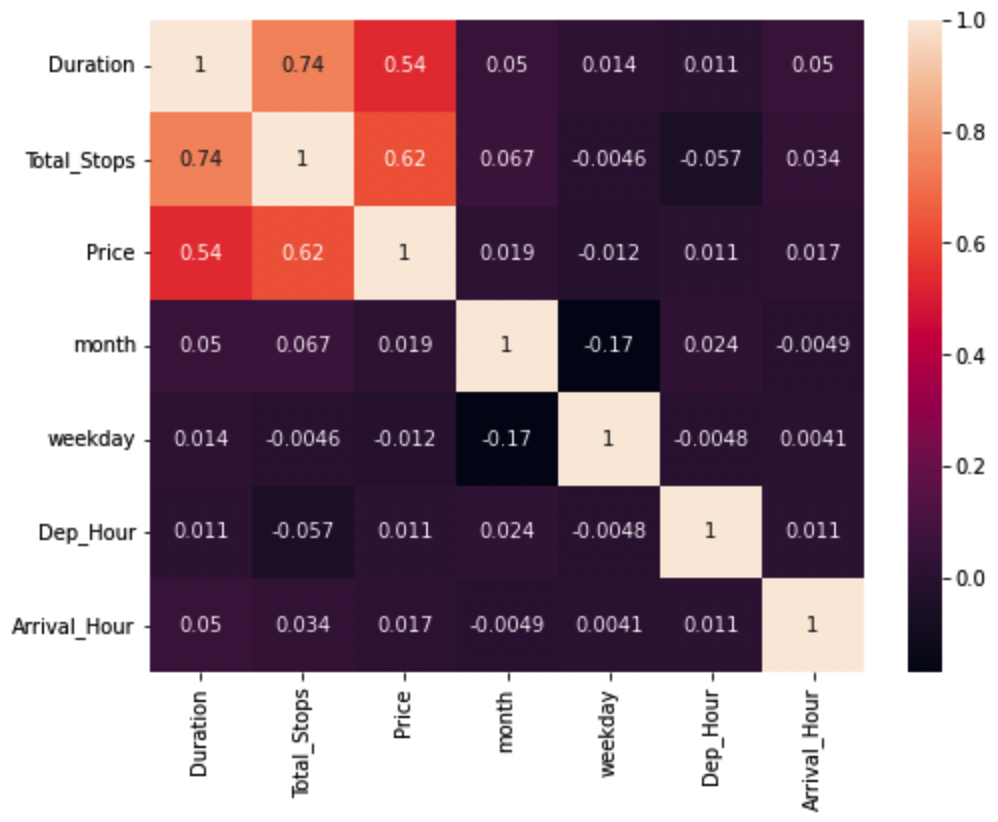
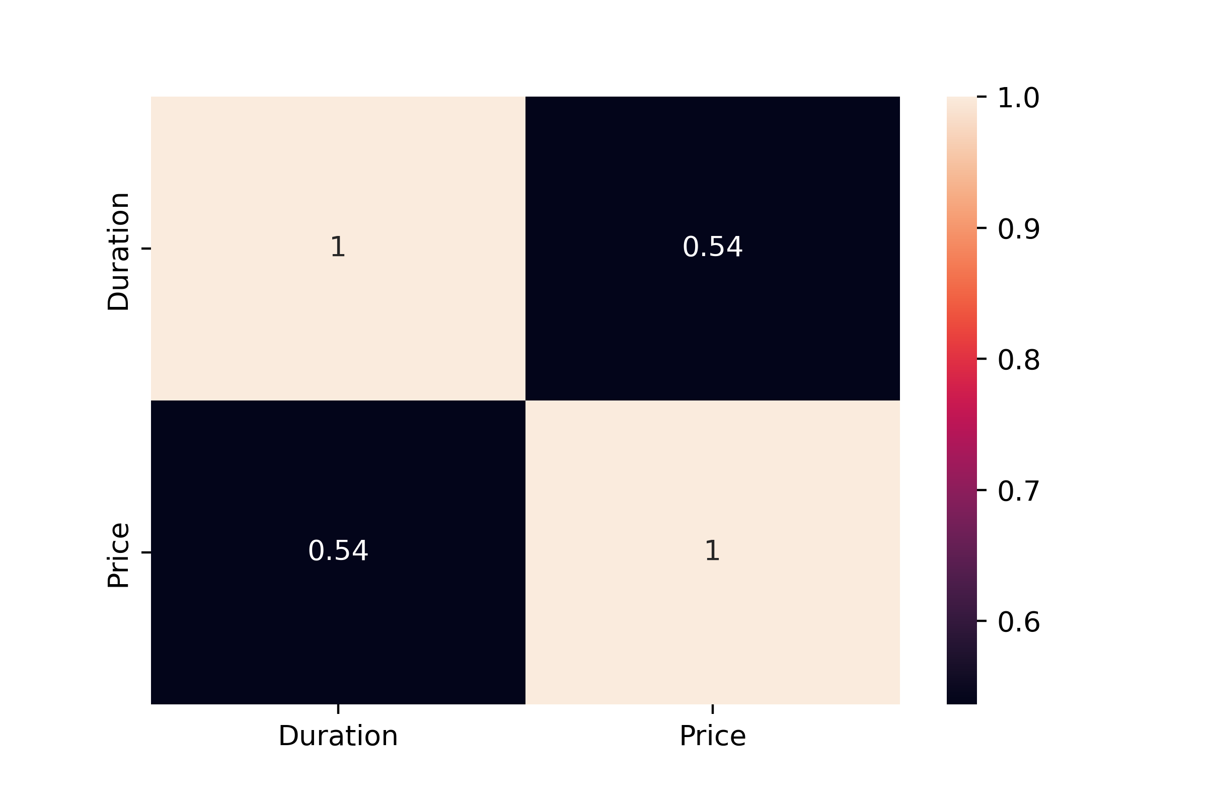
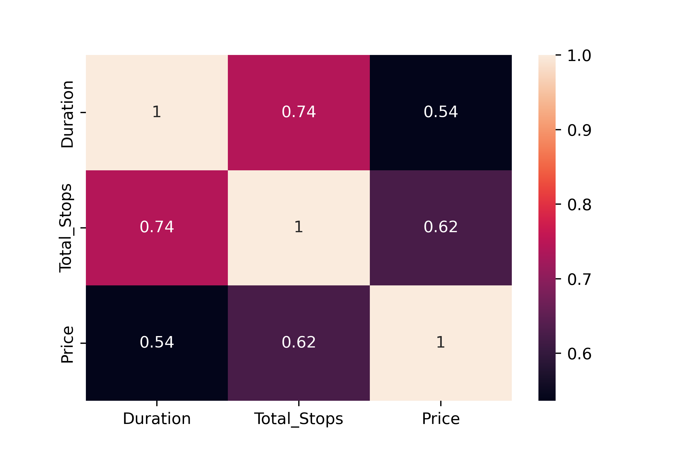
Corrélation
pd.cut()
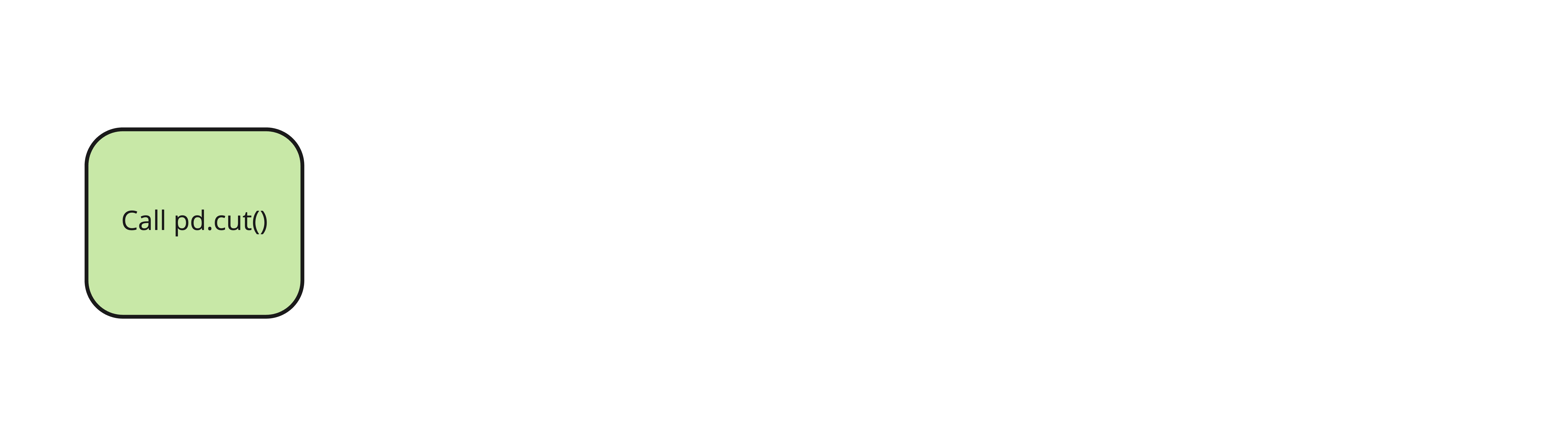
planes["Price_Category"] = pd.cut(
pd.cut()
planes["Price_Category"] = pd.cut(planes["Price"],
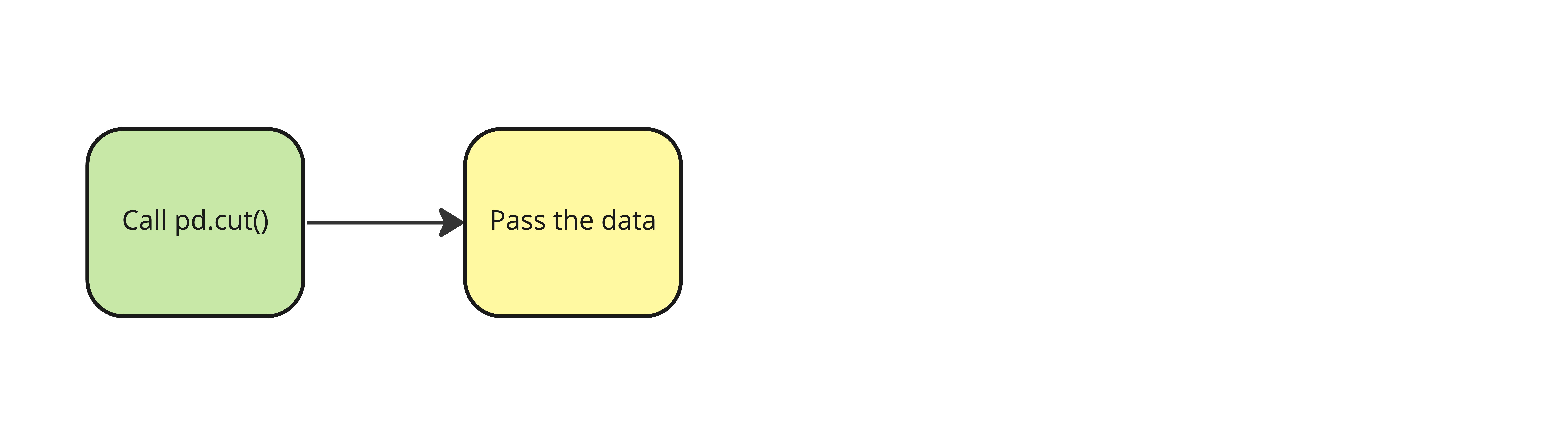
pd.cut()
planes["Price_Category"] = pd.cut(planes["Price"],
                                  labels=labels,
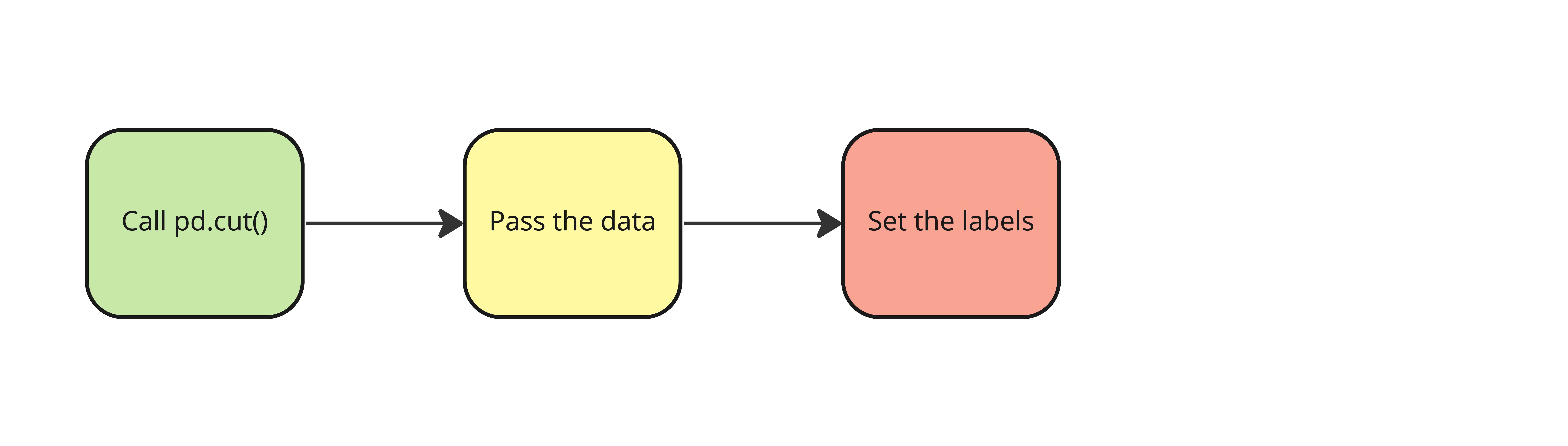
pd.cut()
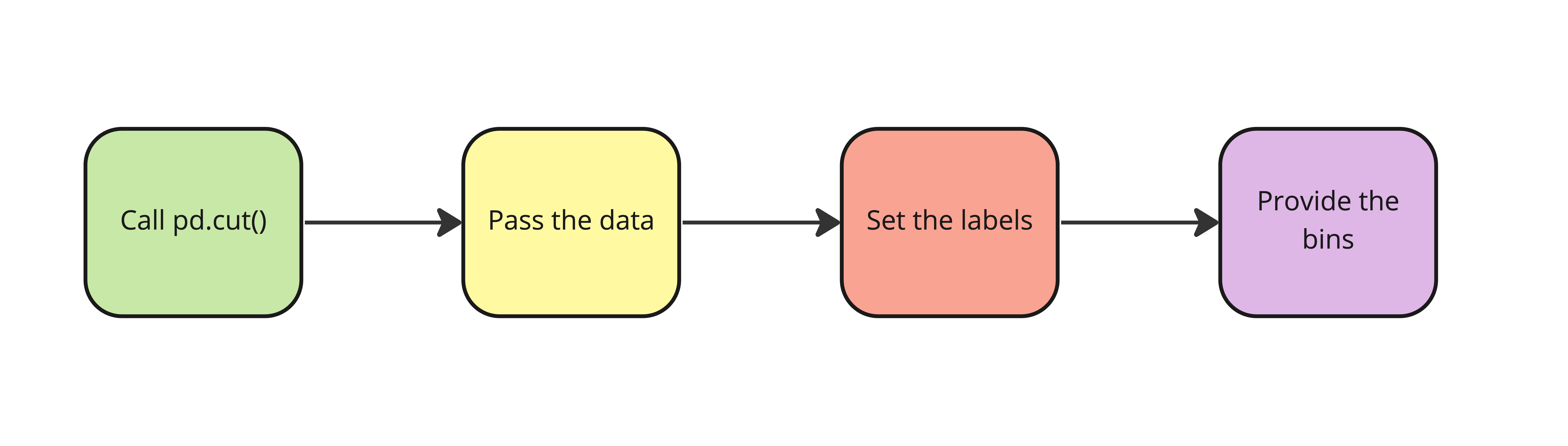
planes["Price_Category"] = pd.cut(planes["Price"],
                                  labels=labels,
                                  bins=bins)
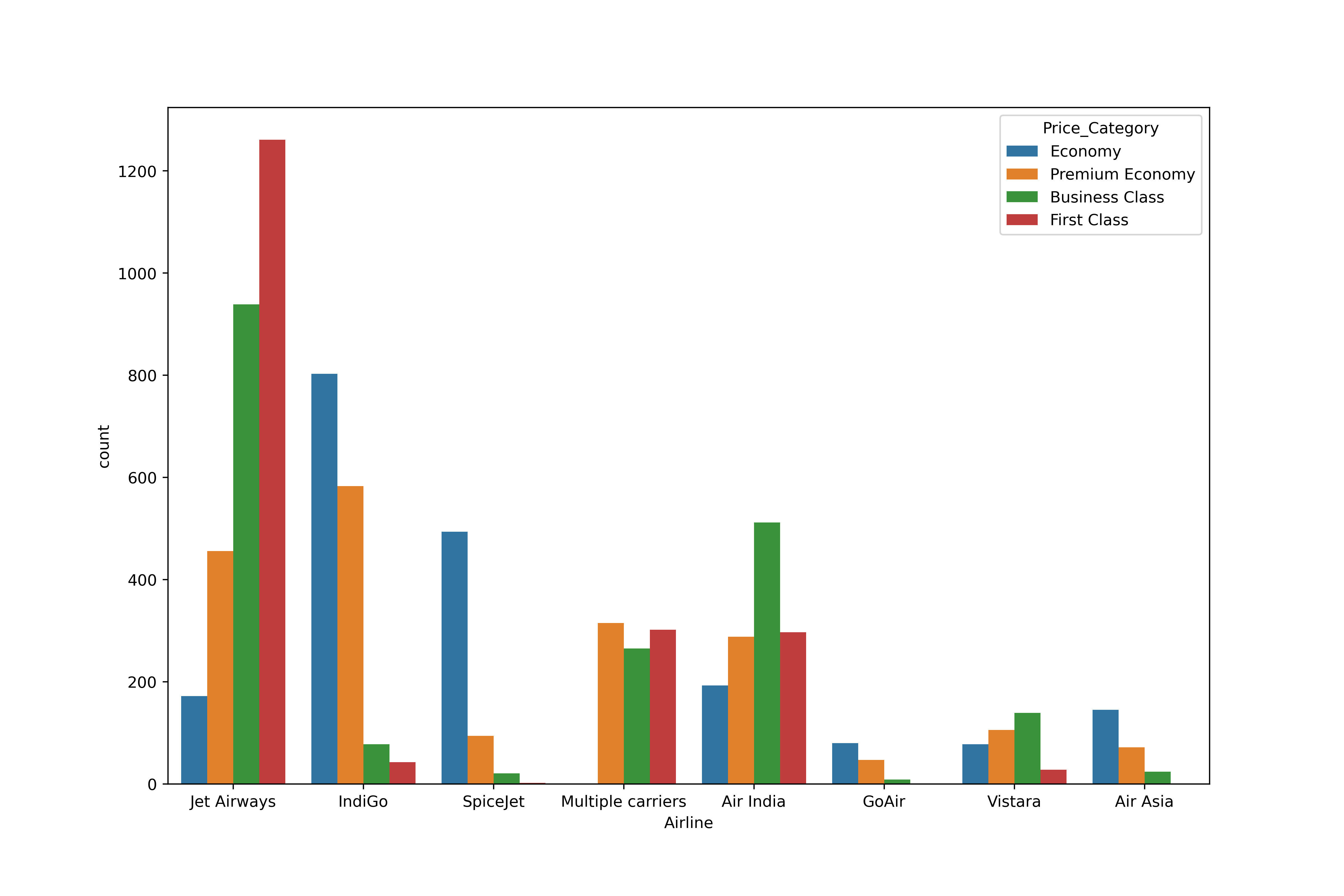
Catégorie de prix par compagnie aérienne

