Mise à jour des paramètres à l’aide des dérivées

Introduction au deep learning avec PyTorch

Jasmin Ludolf

Senior Data Science Content Developer, DataCamp

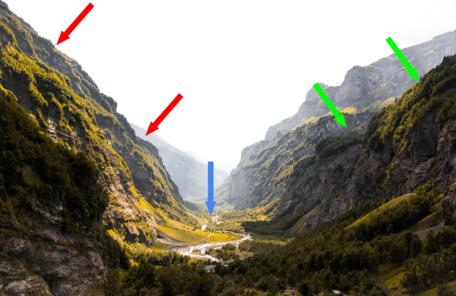
Une analogie pour les dérivées

La dérivée représente la pente de la courbe

Pentes raides (flèches rouges) :
- Grandes pas, dérivée élevée
Pentes plus douces (flèches vertes) :
- Petits pas, dérivée faible
Fond de la vallée (flèche bleue) :
- Plat, dérivée nulle

l’image d’une vallée

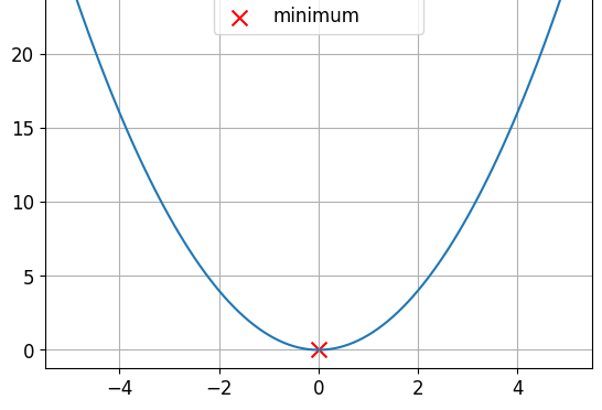
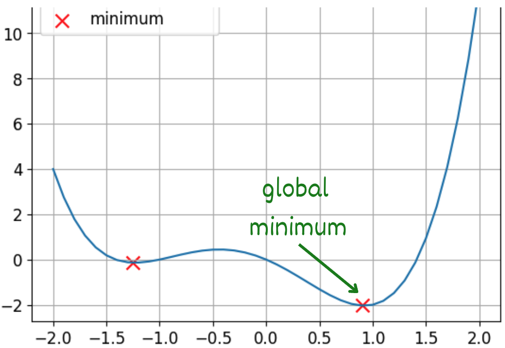
Fonctions convexes et non convexes

Il s’agit d’une fonction convexe

exemple de fonction convexe

Il s’agit d’une fonction non convexe

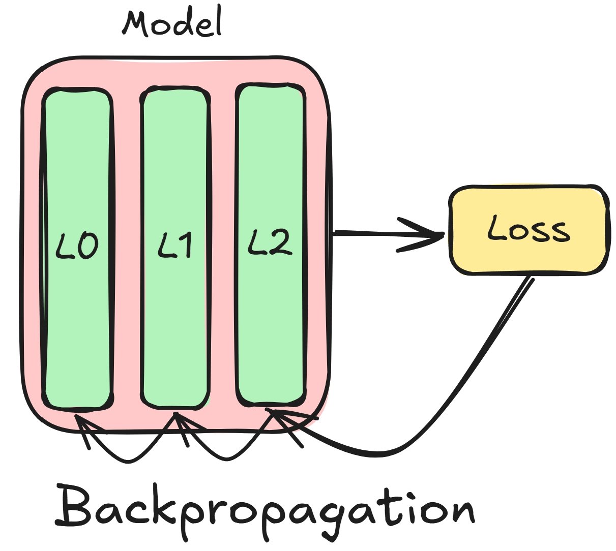
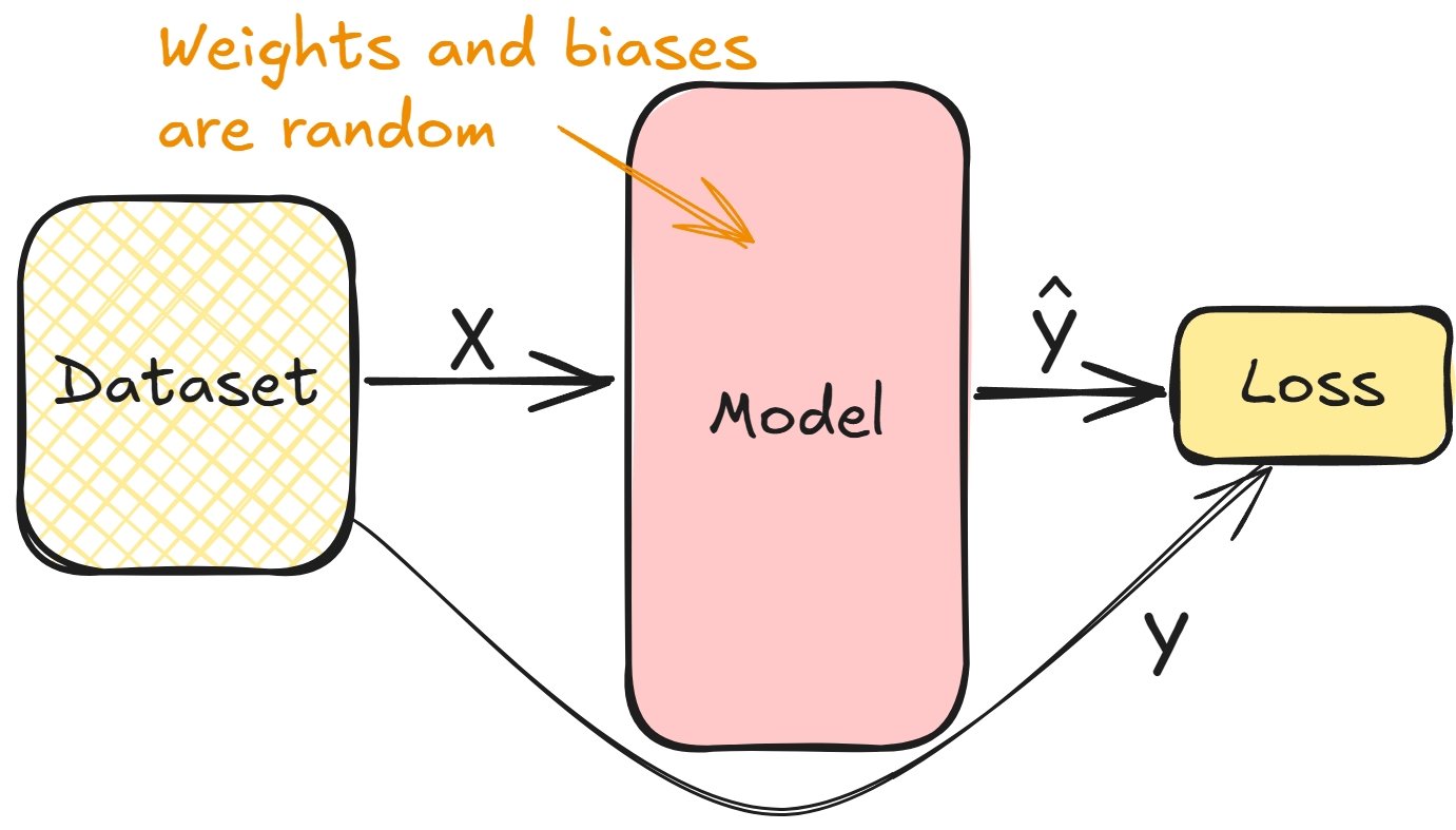
exemple de fonction non convexe avec un minimum global mis en évidence

Relier les dérivées et l’entraînement du modèle

Calculer la perte lors du passage avant pendant l’entraînement

$$ Calcul de la perte

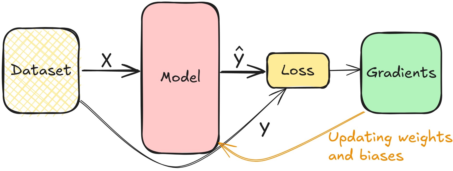
Relier les dérivées et l’entraînement du modèle

Les gradients permettent de minimiser la perte, d’ajuster les poids des couches et les biais
Répétez l’opération jusqu’à ce que les couches soient ajustées

$$ Calcul des gradients

Concepts de rétropropagation

Considérons un réseau composé de trois couches :
- Commencer par des gradients de perte pour $L2$
- Utiliser $L2$ pour calculer les gradients de $L1$
- Répéter l’opération pour toutes les couches ($L1$, $L0$)

Schéma de rétropropagation

La rétropropagation dans PyTorch

# Run a forward pass 
model = nn.Sequential(nn.Linear(16, 8),
                      nn.Linear(8, 4),
                      nn.Linear(4, 2))
prediction = model(sample)


# Calculate the loss and gradients
criterion = CrossEntropyLoss()
loss = criterion(prediction, target)
loss.backward()

# Access each layer's gradients
model[0].weight.grad
model[0].bias.grad
model[1].weight.grad
model[1].bias.grad
model[2].weight.grad
model[2].bias.grad

Mise à jour manuelle des paramètres du modèle

# Learning rate is typically small
lr = 0.001

# Update the weights
weight = model[0].weight
weight_grad = model[0].weight.grad


weight = weight - lr * weight_grad


# Update the biases
bias = model[0].bias
bias_grad = model[0].bias.grad

bias = bias - lr * bias_grad

Accéder au gradient de chaque couche
Multiplier par le taux d’apprentissage
Soustraire ce produit au poids

Descente de gradient

Pour les fonctions non convexes, nous utiliserons la descente de gradient
PyTorch simplifie cela grâce à des optimiseurs
- Descente de gradient stochastique (SGD)

import torch.optim as optim

# Create the optimizer
optimizer = optim.SGD(model.parameters(), lr=0.001)


# Perform parameter updates
optimizer.step()

Passons à la pratique !

Introduction au deep learning avec PyTorch