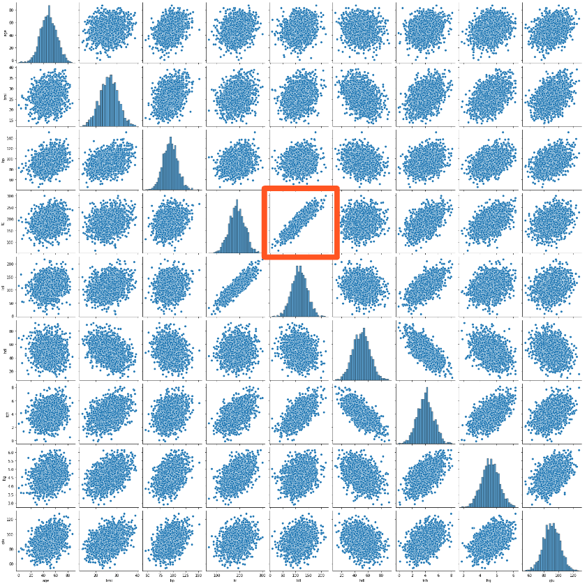
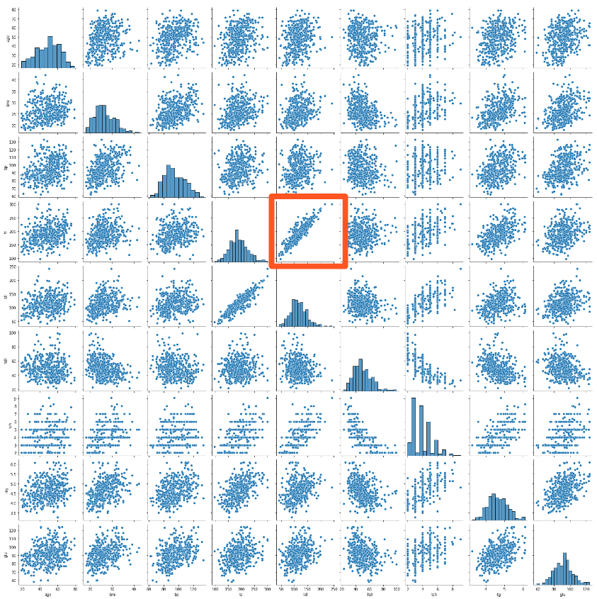
Inputs with correlations
Monte Carlo Simulations in Python

Izzy Weber
Curriculum Manager, DataCamp
Pairplot of simulation results
# Simulated results
sns.pairplot(df_results)
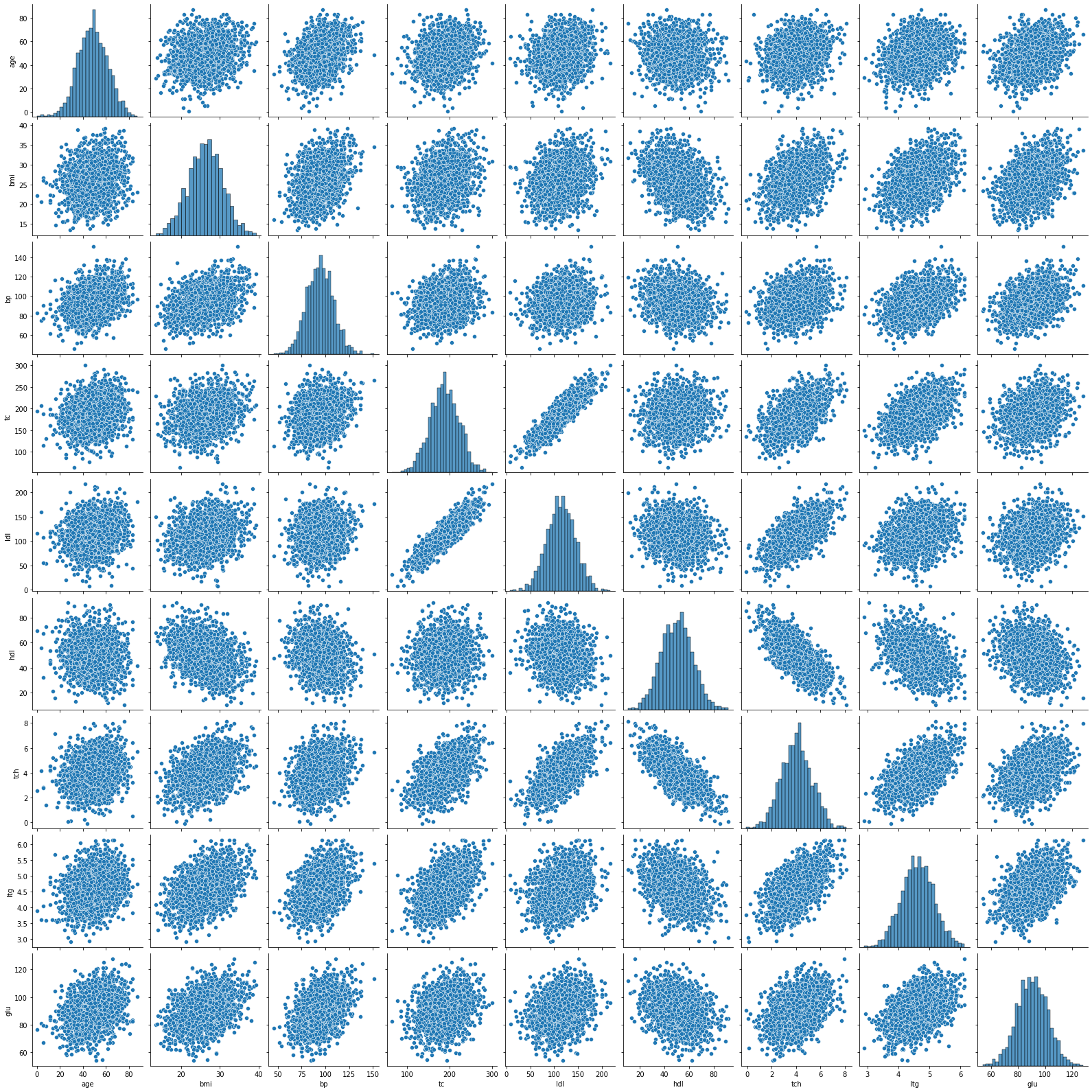
sns.pairplot(dia[["age", "bmi", "bp", "tc", "ldl",
                  "hdl", "tch", "ltg", "glu"]])
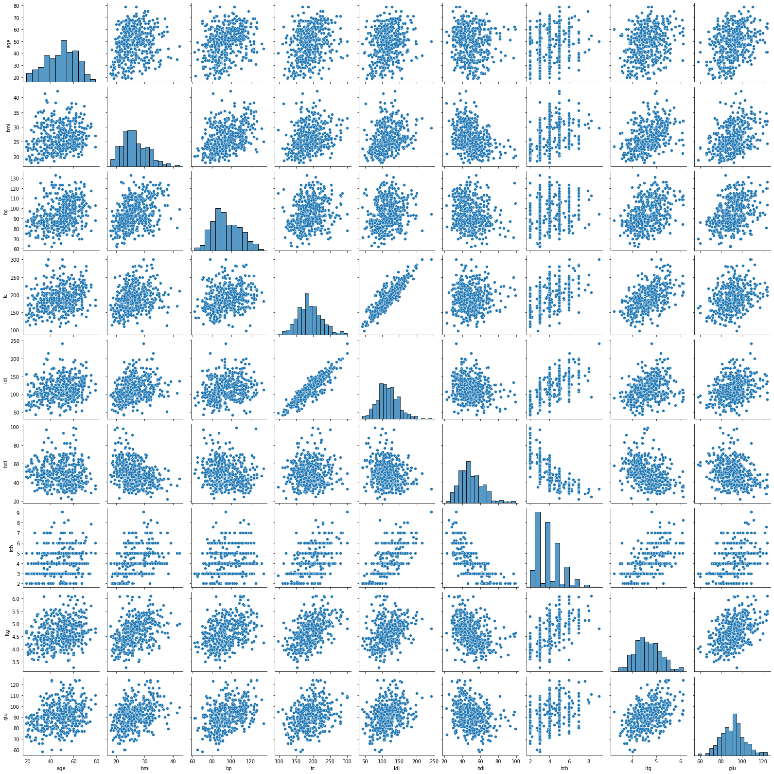
Pairplot of simulation results
# Simulated results
sns.pairplot(df_results)
sns.pairplot(dia[["age", "bmi", "bp", "tc", "ldl",
                  "hdl", "tch", "ltg", "glu"]])
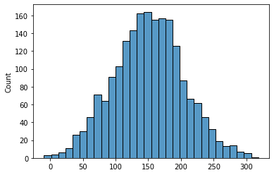
Histogram of the predicted y
sns.histplot(predicted_y)