Diagrammes linéaires

Introduction à la visualisation de données avec ggplot2

Rick Scavetta

Founder, Scavetta Academy

Types de graphiques courants

Type de graphique Geoms possibles
Diagrammes en nuages de points points, jitter, abline, smooth, count
Diagrammes à barres histogram, bar, col, errorbar
Diagrammes linéaires line, path
Introduction à la visualisation de données avec ggplot2

Castor

str(beaver)
'data.frame':    101 obs. of  3 variables:
 $ time  : POSIXct, format: "2000-01-01 09:30:00" "2000-01-01 09:40:00" "2000-01-01 09:50:00" ...
 $ temp  : num  36.6 36.7 36.9 37.1 37.2 ...
 $ active: Factor w/ 2 levels "0","1": 1 1 1 1 1 1 1 1 1 1 ...
Introduction à la visualisation de données avec ggplot2

Castor

ggplot(beaver, aes(x = time, y = temp)) +
  geom_line()

Introduction à la visualisation de données avec ggplot2

Castor

ggplot(beaver, aes(x = time, y = temp, 
                   color = factor(active))
                   ) +
  geom_line()

Introduction à la visualisation de données avec ggplot2

Ensemble de données sur les prises de poissons

str(fish)
'data.frame':    427 obs. of  3 variables:
 $ Species: Factor w/ 7 levels "Pink","Chum",..: 1 2 3 4 5 6 7 1 2 3 ...
 $ Year   : int  1950 1950 1950 1950 1950 1950 1950 1951 1951 1951 ...
 $ Capture: int  100600 139300 64100 30500 0 23200 10800 259000 155900 51200 ...
Introduction à la visualisation de données avec ggplot2

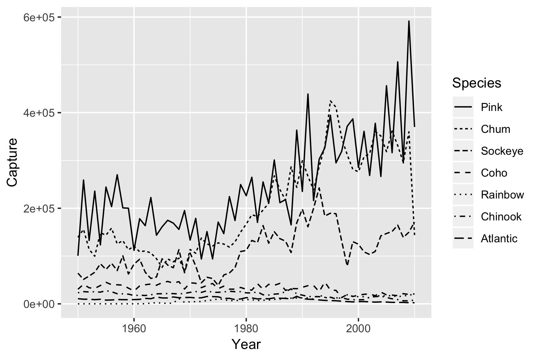
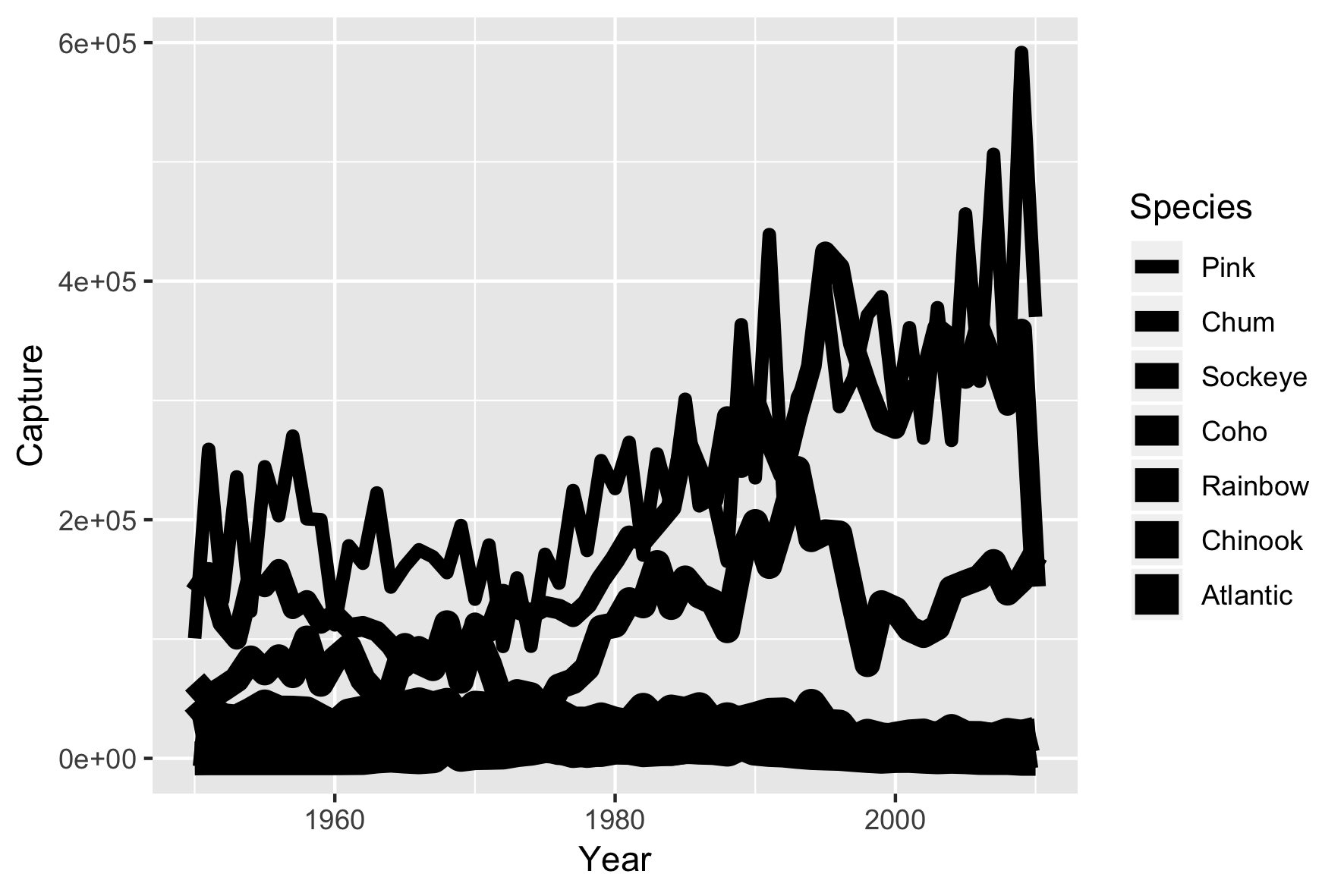
Attribut esthétique linetype

ggplot(fish, aes(x = Year, 
                 y = Capture, 
                 linetype = Species)) + 
  geom_line()

Introduction à la visualisation de données avec ggplot2

Attribut esthétique size

ggplot(fish, aes(x = Year, 
                 y = Capture, 
                 size = Species)) + 
  geom_line()

Introduction à la visualisation de données avec ggplot2

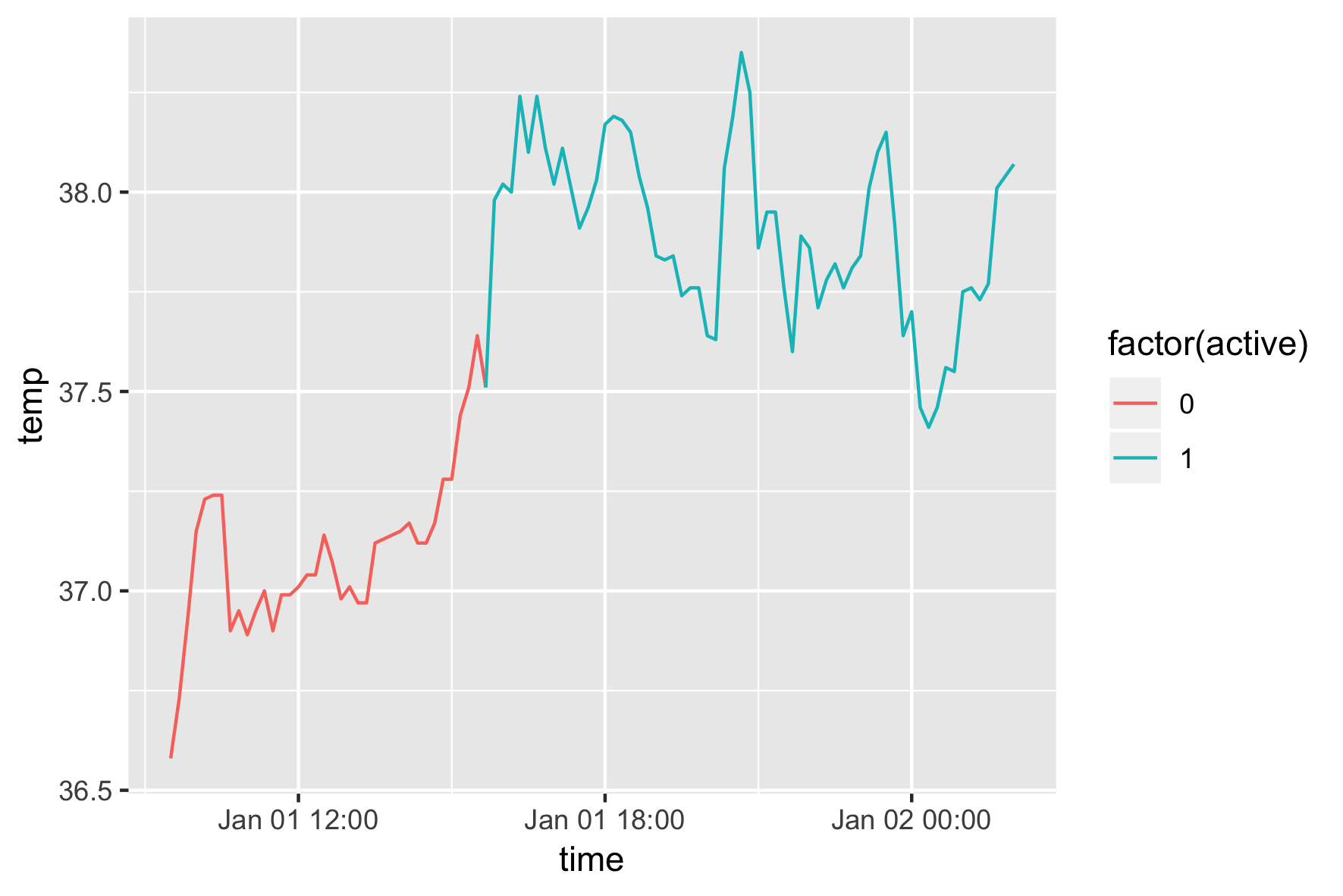
Attribut esthétique color

ggplot(fish, aes(x = Year, 
                 y = Capture, 
                 color = Species)) + 
  geom_line()

Introduction à la visualisation de données avec ggplot2

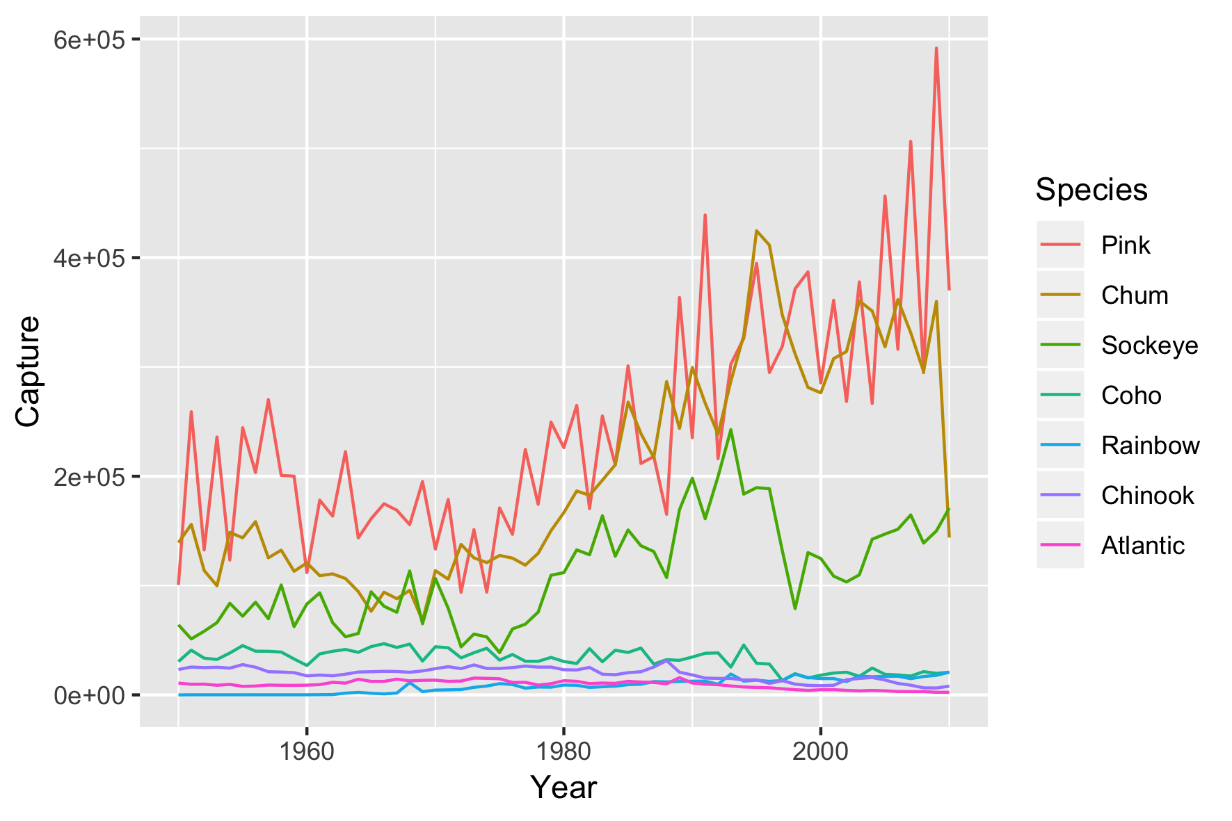
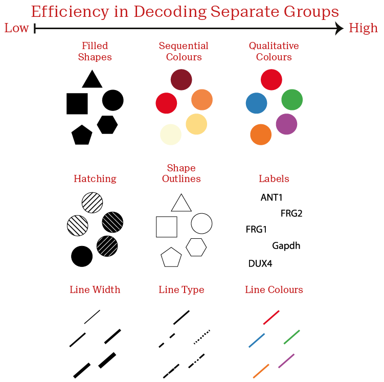
Attributs esthétiques pour les variables catégorielles

Introduction à la visualisation de données avec ggplot2

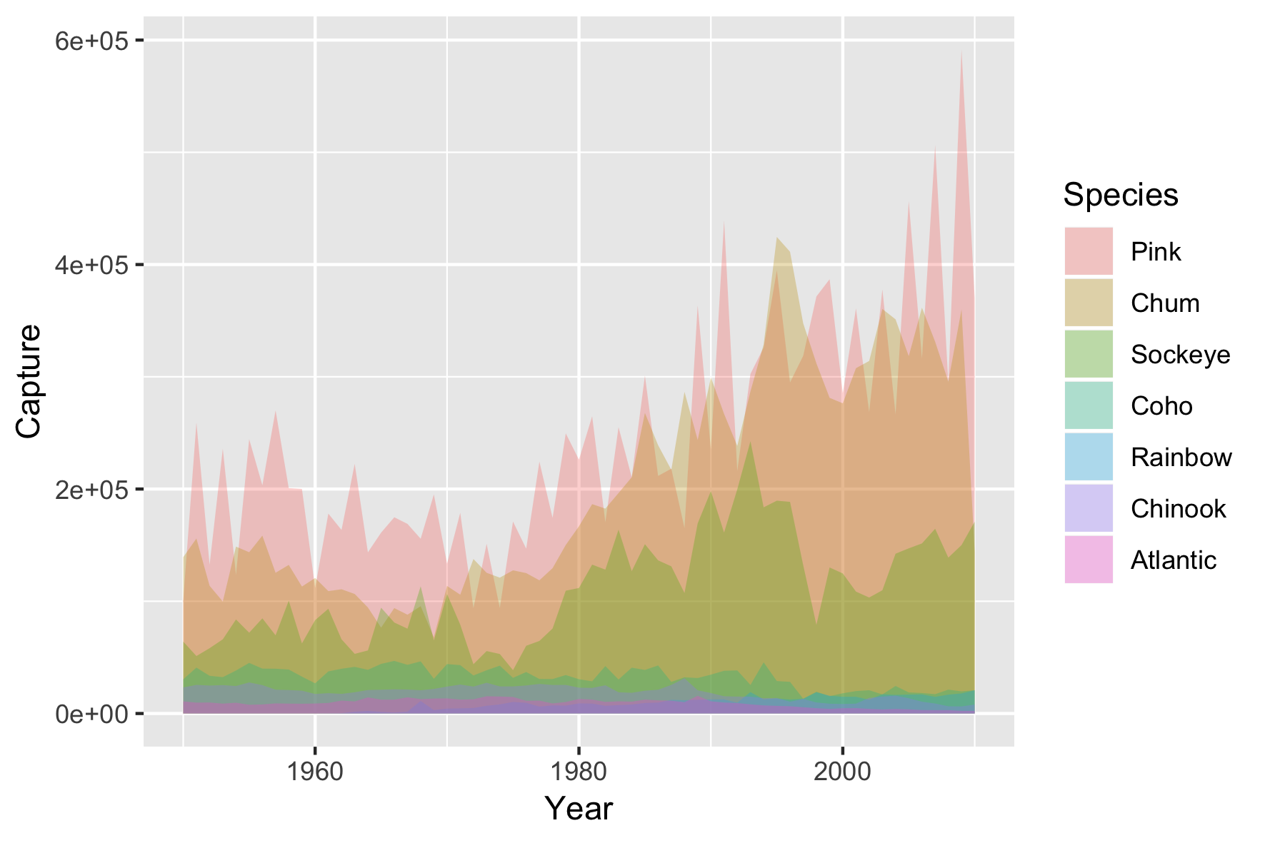
Attribut esthétique fill avec geom_area()

ggplot(fish, aes(x = Year, 
                 y = Capture, 
                 fill = Species)) + 
  geom_area()

Introduction à la visualisation de données avec ggplot2

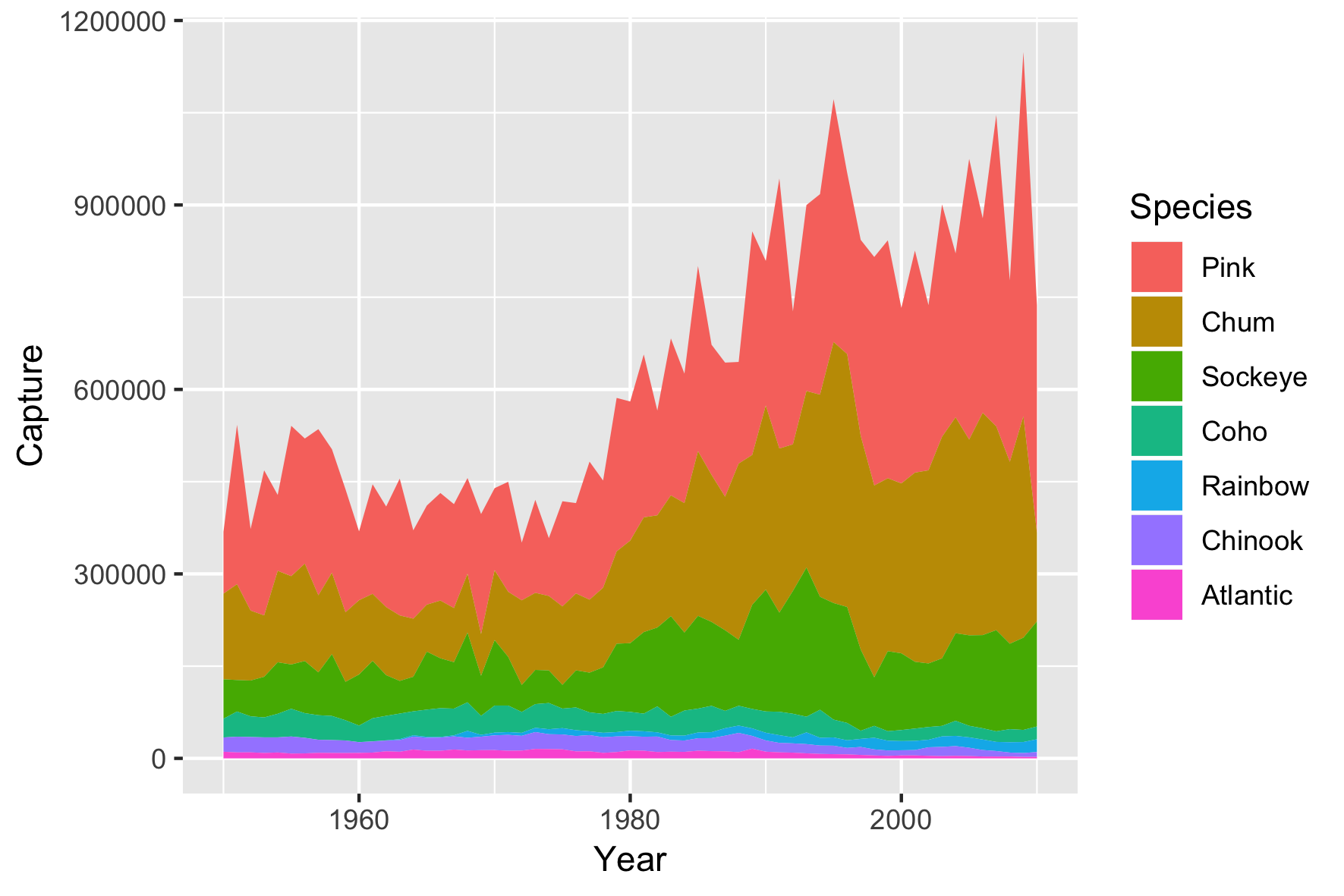
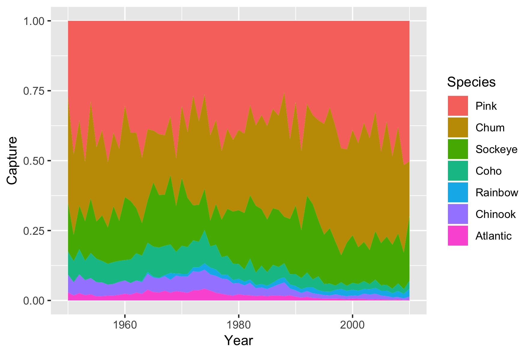
Utilisation de position = "fill"

ggplot(fish, aes(x = Year, 
                 y = Capture, 
                 fill = Species)) + 
  geom_area(position = "fill")

Introduction à la visualisation de données avec ggplot2

geom_ribbon()

ggplot(fish, aes(x = Year, 
                 y = Capture, 
                 fill = Species)) + 
  geom_ribbon(aes(ymax = Capture, 
                  ymin = 0), 
              alpha = 0.3)

Introduction à la visualisation de données avec ggplot2

Passons à la pratique !

Introduction à la visualisation de données avec ggplot2

Preparing Video For Download...