Modification des attributs esthétiques
Introduction à la visualisation de données avec ggplot2

Rick Scavetta
Founder, Scavetta Academy
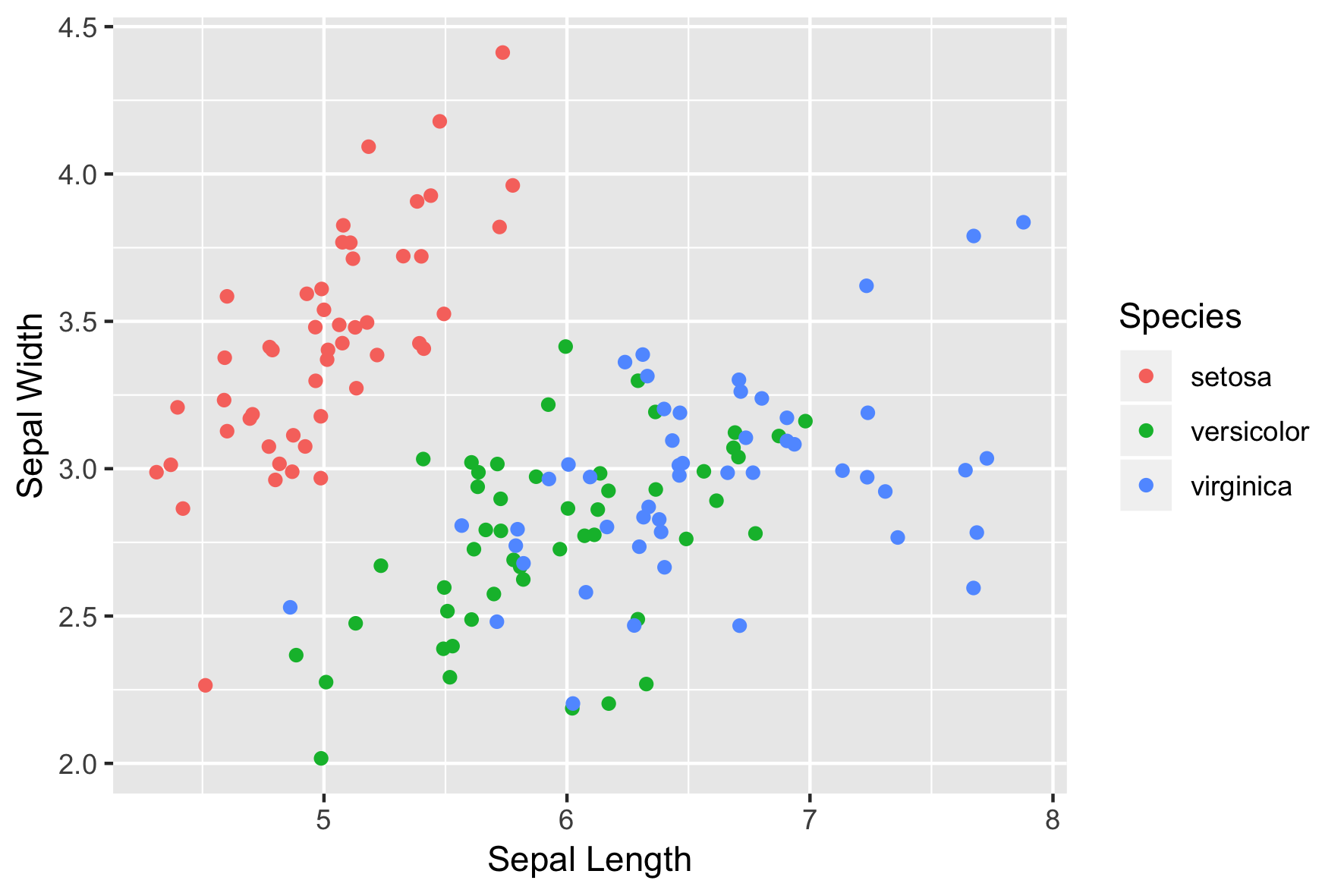
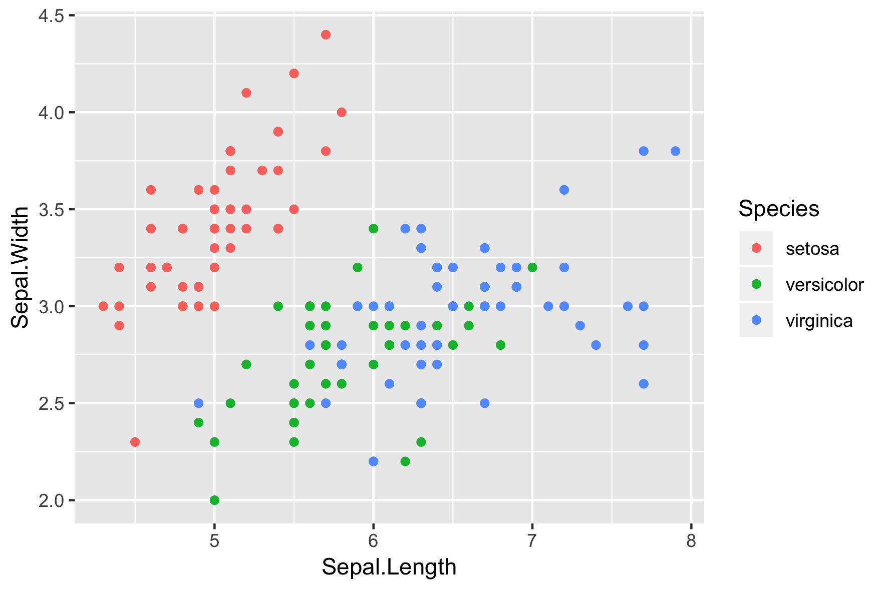
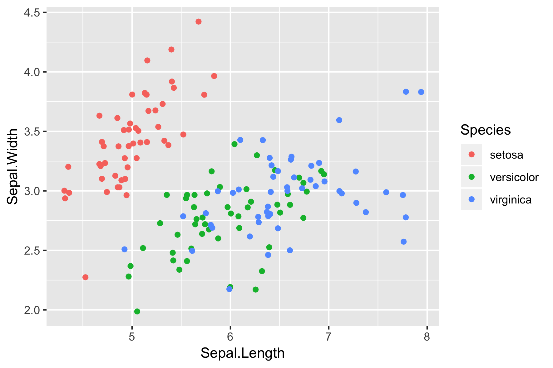
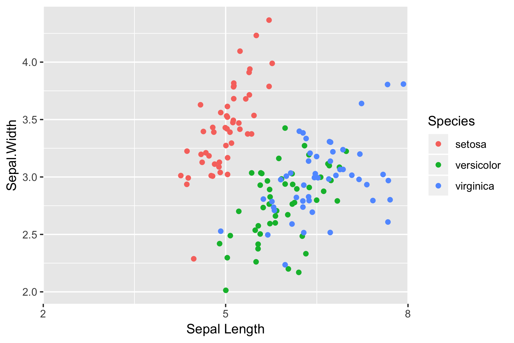
position = "identity" (default)

position = "identity" (default)
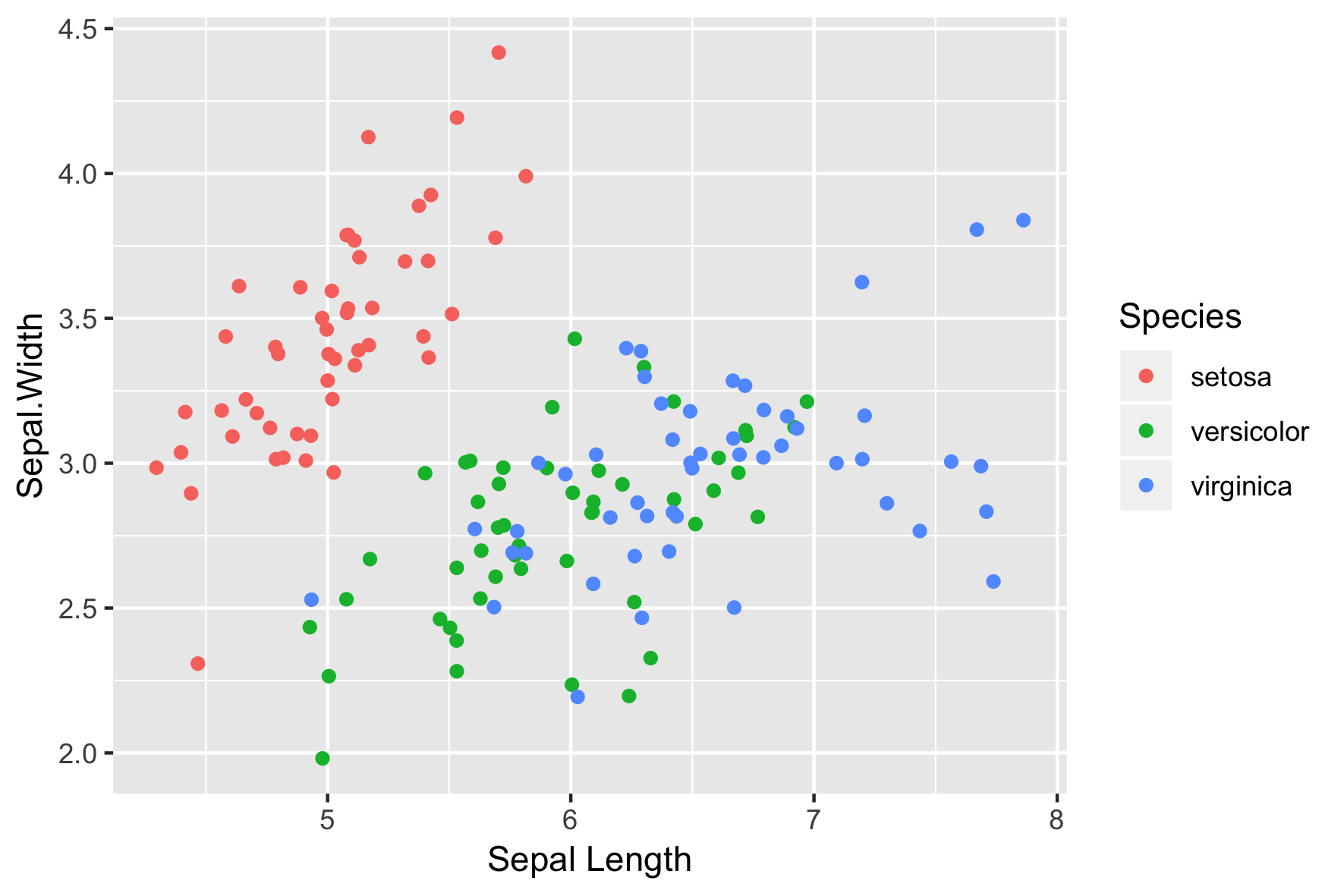
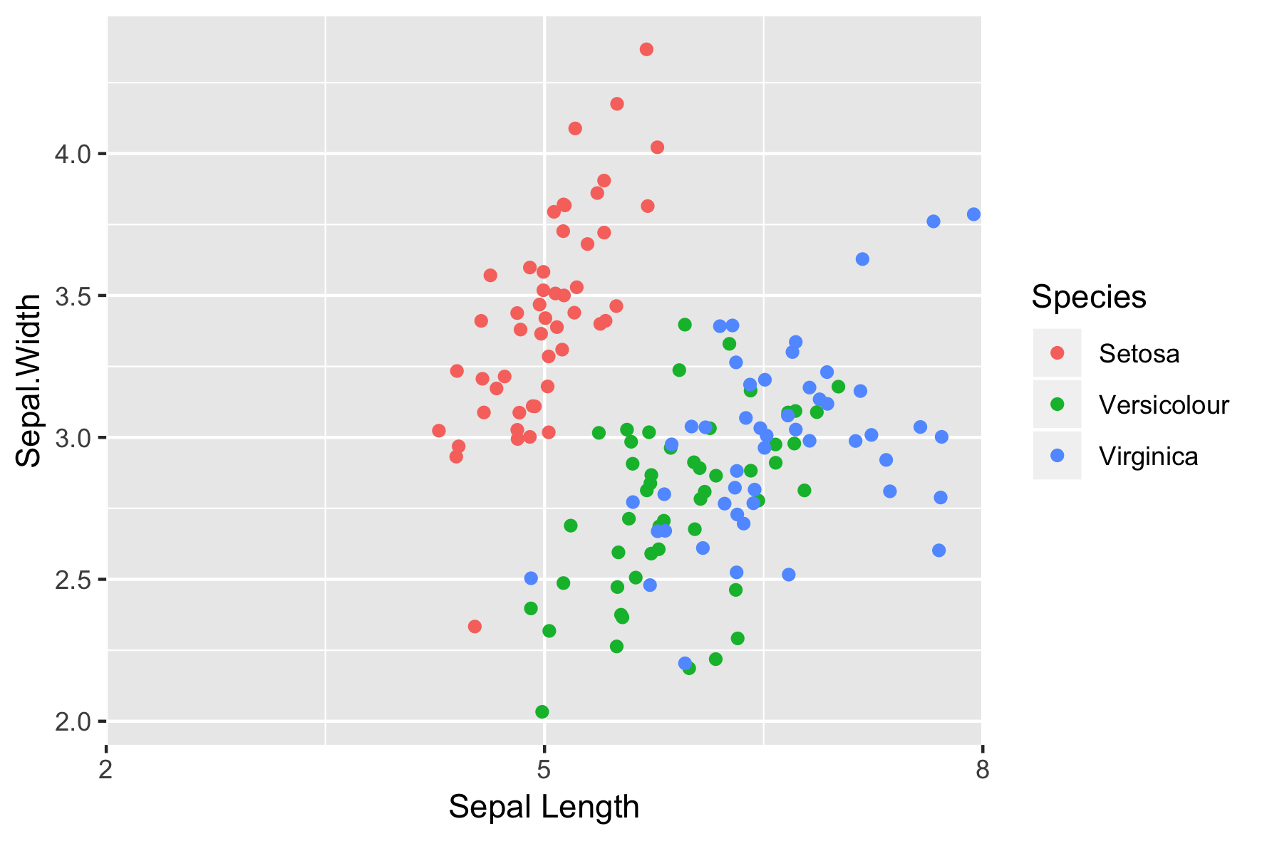
position = "jitter"
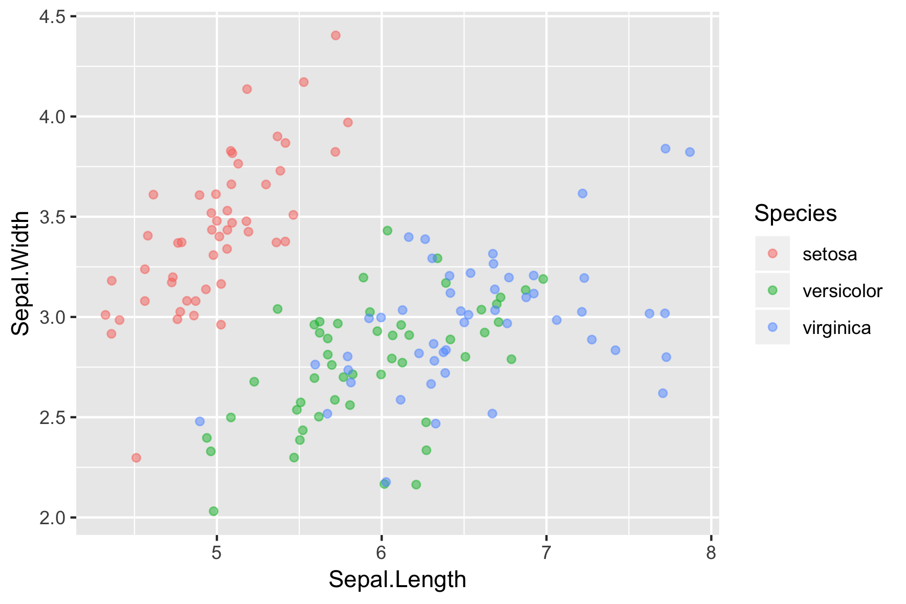
position_jitter()
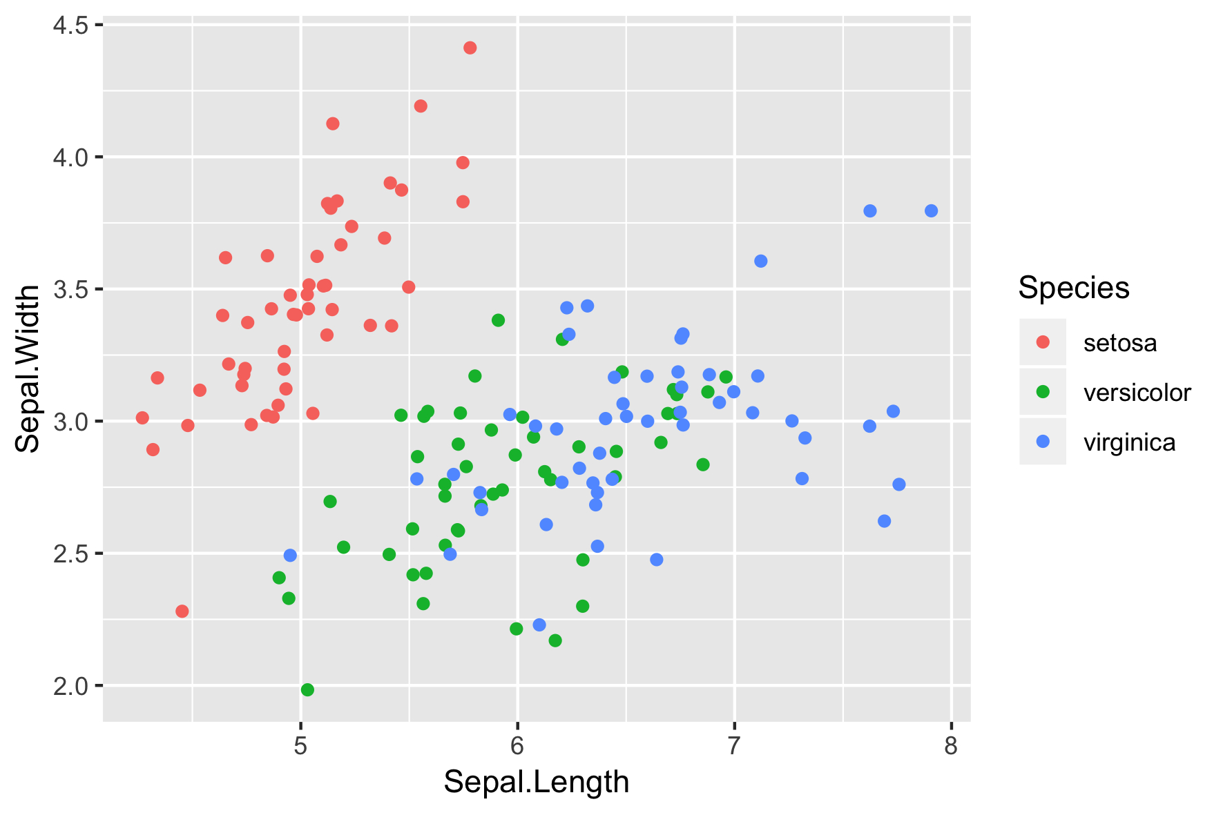
position_jitter()
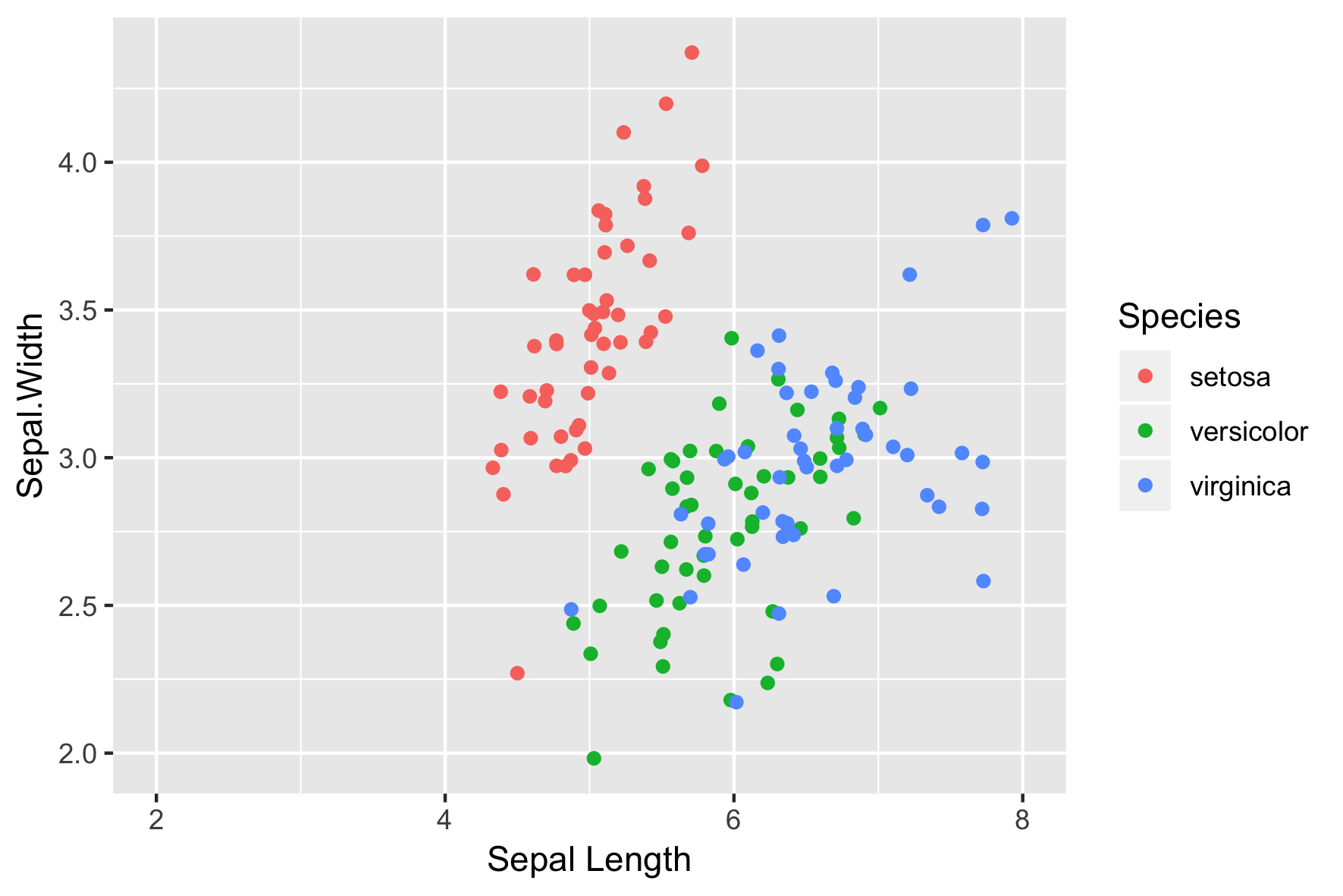
scale_*_*()
L'argument limits
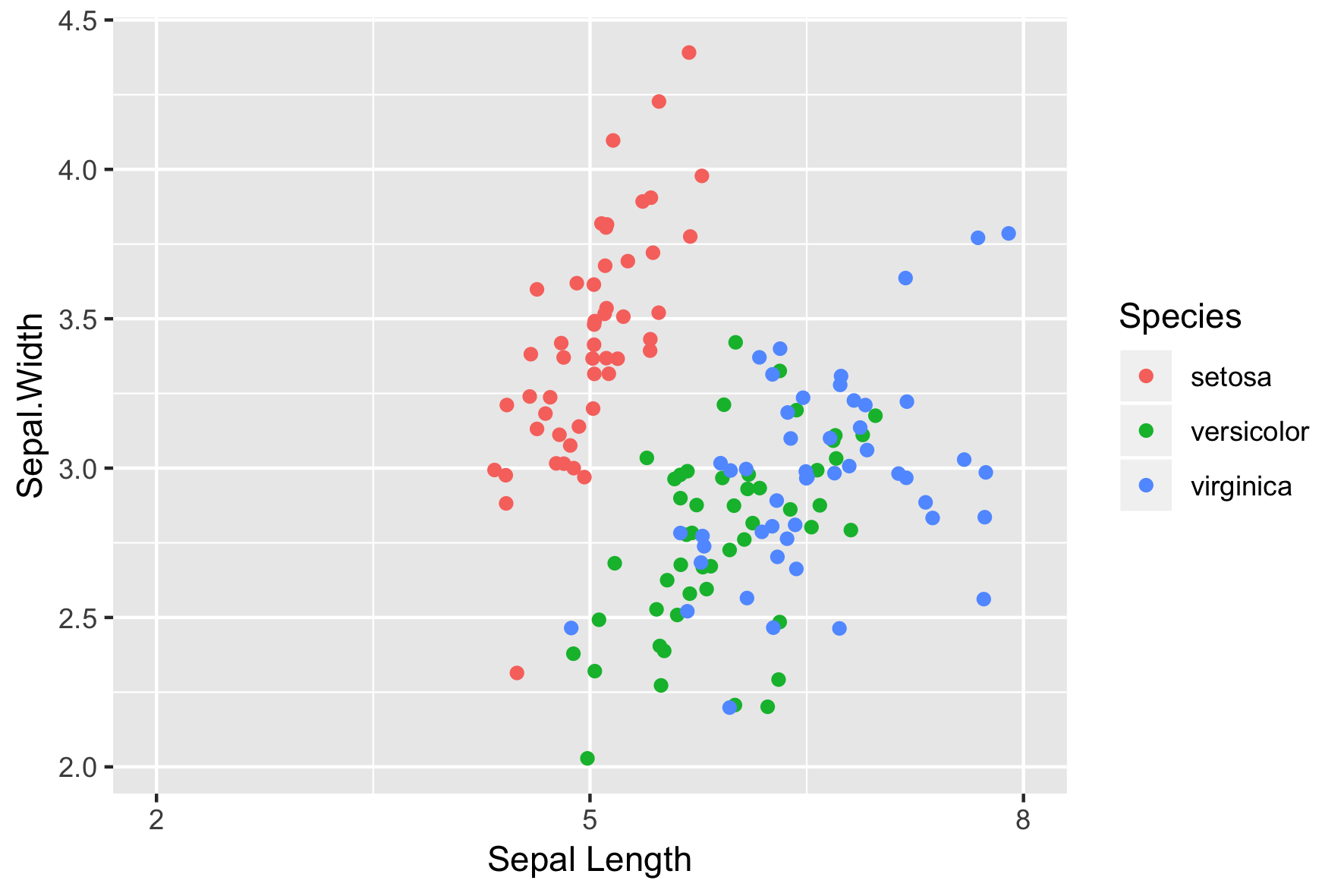
L'argument breaks
L'argument expand
L'argument labels
labs()