Pourquoi la régression logistique est-elle nécessaire ?
Introduction à la régression avec statsmodels en Python

Maarten Van den Broeck
Content Developer at DataCamp
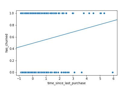
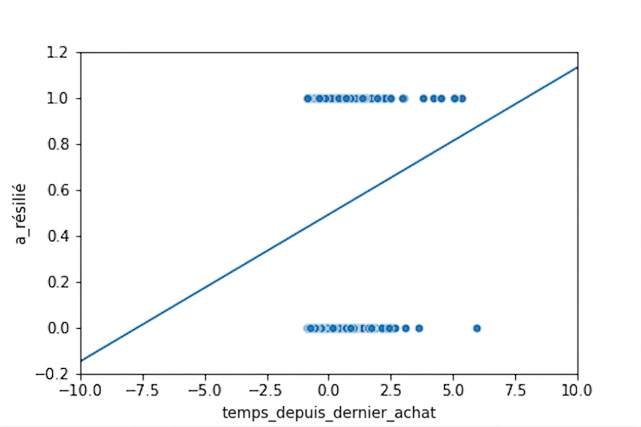
Visualisation du modèle linéaire
Zoom arrière
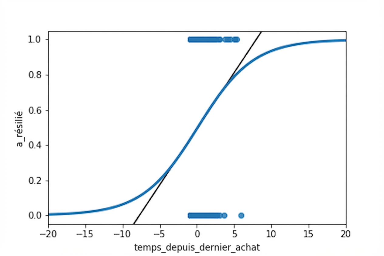
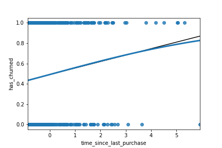
Visualisation du modèle logistique
Zoom arrière