Pourquoi la régression logistique est-elle nécessaire ?
Introduction à la régression dans R

Richie Cotton
Data Evangelist at DataCamp
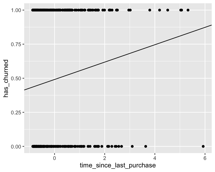
Visualisation du modèle linéaire
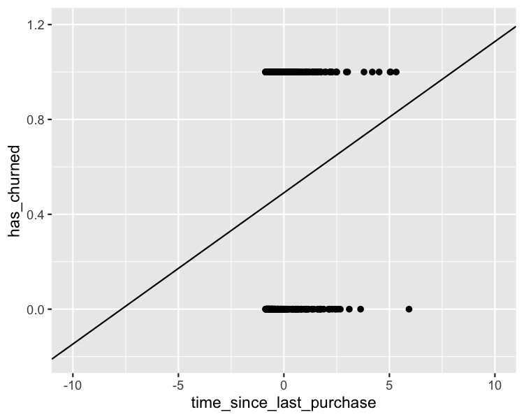
Zoom arrière
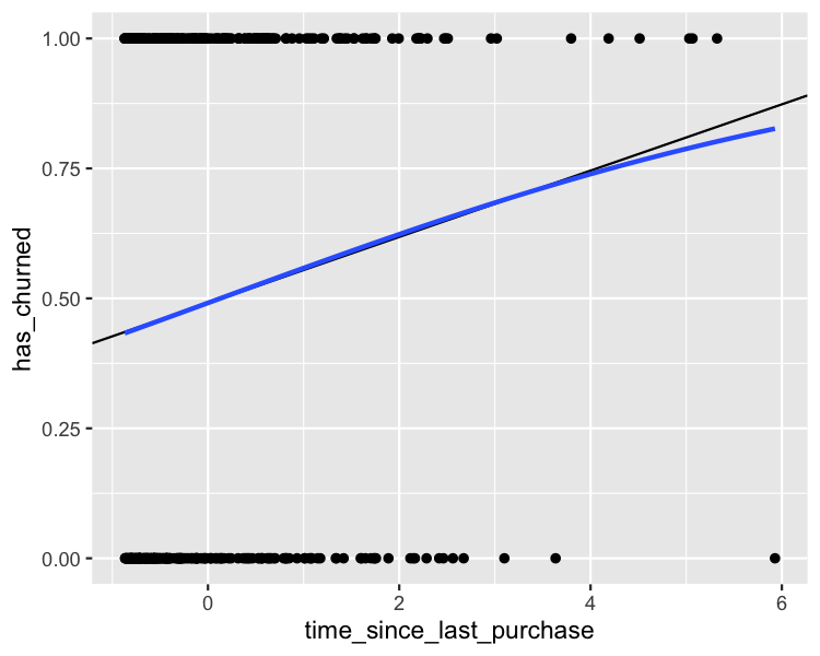
Visualisation du modèle logistique
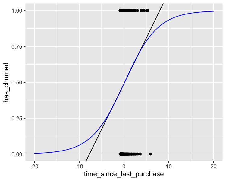
Zoom arrière
Introduction à la régression dans R
Richie Cotton
Data Evangelist at DataCamp

