Valeurs aberrantes, levier et influence

Introduction à la régression dans R

Richie Cotton

Data Evangelist at DataCamp

Ensemble de données sur les gardons

roach <- fish %>%
  filter(species == "Roach")

species	length_cm	mass_g
Gardon	12,9	40
Gardon	16,5	69
Gardon	17,5	78
Gardon	18,2	87
Gardon	18,6	120
...	...	...

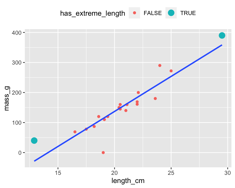
Quels points sont des valeurs aberrantes ?

ggplot(roach, aes(length_cm, mass_g)) +
  geom_point() +
  geom_smooth(method = "lm", se = FALSE)

Diagramme en nuage de points représentant la masse des gardons en fonction de leur longueur, avec une courbe de tendance. La plupart des points suivent de près la courbe de tendance.

Valeurs explicatives extrêmes

roach %>% 
  mutate(
    has_extreme_length = length_cm < 15 | length_cm > 26
  ) %>% 
  ggplot(aes(length_cm, mass_g)) +
  geom_point(aes(color = has_extreme_length)) +
  geom_smooth(method = "lm", se = FALSE)

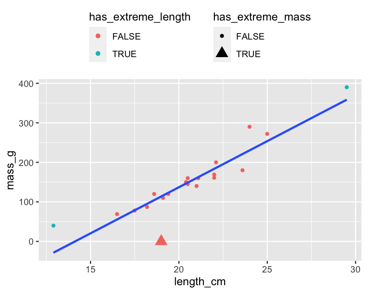
Valeurs de réponse éloignées de la ligne de régression

roach %>% 
  mutate(
    has_extreme_length = length_cm < 15 | length_cm > 26,
    has_extreme_mass = mass_g < 1
  ) %>% 
  ggplot(aes(length_cm, mass_g)) +
  geom_point(
    aes(
      color = has_extreme_length, 
      shape = has_extreme_mass
    )
  ) +
  geom_smooth(method = "lm", se = FALSE)

Diagramme en nuage de points représentant la masse des gardons en fonction de leur longueur, avec une courbe de tendance. La plupart des points sont de couleur rouge, mais un gardon très court et un gardon très long ont des points de couleur cyan. La plupart des points sont des cercles, mais un point représentant un poisson dont la masse apparente est nulle est un triangle.

Levier

Le levier est une mesure de l'extrême variation des valeurs des variables explicatives.

mdl_roach <- lm(mass_g ~ length_cm, data = roach)

hatvalues(mdl_roach)

     1      2      3      4      5      6      7 
0.3137 0.1255 0.0935 0.0763 0.0684 0.0619 0.0605 
     8      9     10     11     12     13     14 
0.0568 0.0503 0.0501 0.0501 0.0506 0.0509 0.0581 
    15     16     17     18     19     20 
0.0581 0.0593 0.0884 0.0995 0.1334 0.3947

La colonne .hat

library(broom)
augment(mdl_roach)

# A tibble: 20 × 8
   mass_g length_cm .fitted   .resid   .hat .sigma   .cooksd .std.resid
    <dbl>     <dbl>   <dbl>    <dbl>  <dbl>  <dbl>     <dbl>      <dbl>
 1     40      12.9   -28.6   68.6   0.314    33.8 1.07          2.17  
 2     69      16.5    55.4   13.6   0.126    39.1 0.0104        0.381 
 3     78      17.5    78.7   -0.711 0.0935   39.3 0.0000197    -0.0196
 4     87      18.2    95.0   -8.03  0.0763   39.2 0.00198      -0.219 
 5    120      18.6   104.    15.6   0.0684   39.1 0.00661       0.424 
...

Gardons à fort levier

mdl_roach %>%
  augment() %>%
  select(mass_g, length_cm, leverage = .hat) %>%
  arrange(desc(leverage)) %>% 
  head()

# A tibble: 6 x 3
  mass_g length_cm leverage
   <dbl>     <dbl>    <dbl>
1    390      29.5   0.395  # really long roach
2     40      12.9   0.314  # really short roach
3    272      25     0.133 
4     69      16.5   0.126 
5    290      24     0.0995
6     78      17.5   0.0935

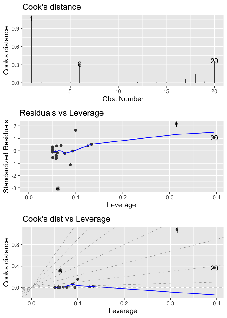
Influence

L'influence mesure dans quelle mesure le modèle changerait si vous retiriez l'observation de l'ensemble de données lors de la modélisation.

Une personne manipulant une clé à molette

Distance de Cook

La distance de Cook est la mesure d'influence la plus couramment utilisée.

cooks.distance(mdl_roach)

       1        2        3        4        5        6 
1.07e+00 1.04e-02 1.97e-05 1.98e-03 6.61e-03 3.12e-01 
       7        8        9       10       11       12 
8.53e-04 1.99e-04 2.57e-04 2.56e-04 2.45e-03 7.95e-03 
      13       14       15       16       17       18 
1.37e-04 4.82e-03 1.15e-02 4.52e-03 6.12e-02 1.50e-01 
      19       20 
2.06e-02 3.66e-01

La colonne *.cooksd

library(broom)
augment(mdl_roach)

# A tibble: 20 x 9
   mass_g length_cm .fitted .se.fit   .resid   .hat .sigma   .cooksd .std.resid
    <dbl>     <dbl>   <dbl>   <dbl>    <dbl>  <dbl>  <dbl>     <dbl>      <dbl>
 1     40      12.9   -28.6   21.4    68.6   0.314    33.8 1.07          2.17  
 2     69      16.5    55.4   13.5    13.6   0.126    39.1 0.0104        0.381 
 3     78      17.5    78.7   11.7    -0.711 0.0935   39.3 0.0000197    -0.0196
 4     87      18.2    95.0   10.5    -8.03  0.0763   39.2 0.00198      -0.219 
 5    120      18.6   104.     9.98   15.6   0.0684   39.1 0.00661       0.424 
...

Les gardons les plus influents

mdl_roach %>%
  augment() %>%
  select(mass_g, length_cm, cooks_dist = .cooksd) %>%
  arrange(desc(cooks_dist)) %>% 
  head()

# A tibble: 6 x 3
  mass_g length_cm cooks_dist
   <dbl>     <dbl>      <dbl>
1     40      12.9     1.07   # really short roach
2    390      29.5     0.366  # really long roach
3      0      19       0.312  # zero mass roach
4    290      24       0.150 
5    180      23.6     0.0612
6    272      25       0.0206

Suppression du gardon le plus influent

roach_not_short <- roach %>% 
  filter(length != 12.9)

ggplot(roach, aes(length_cm, mass_g)) +
  geom_point() +
  geom_smooth(method = "lm", se = FALSE) +
  geom_smooth(
    method = "lm", se = FALSE, 
    data = roach_not_short, color = "red"
  )

![Diagramme en nuage de points représentant la masse des gardons en fonction de leur longueur, avec deux courbes de tendance. Une courbe de tendance utilise toutes les données, tandis qu'une autre exclut le gardon le plus court. Cette deuxième courbe de tendance présente une pente nettement plus raide.

autoplot()

autoplot(
  mdl_roach, 
  which = 4:6, 
  nrow = 3,
  ncol = 1
)

Les trois diagrammes diagnostiques du modèle de gardon, organisés en trois panneaux.

Passons à la pratique !

Introduction à la régression dans R