Introduction au bootstrap

Échantillonnage en R

Richie Cotton

Data Evangelist at DataCamp

Avec ou sans

Échantillonnage sans remise

Des cartes à jouer sur une table de casino.

Échantillonnage avec remise (« rééchantillonnage »)

Quatre dés en train de rouler.

Échantillonnage aléatoire simple sans remise

Population

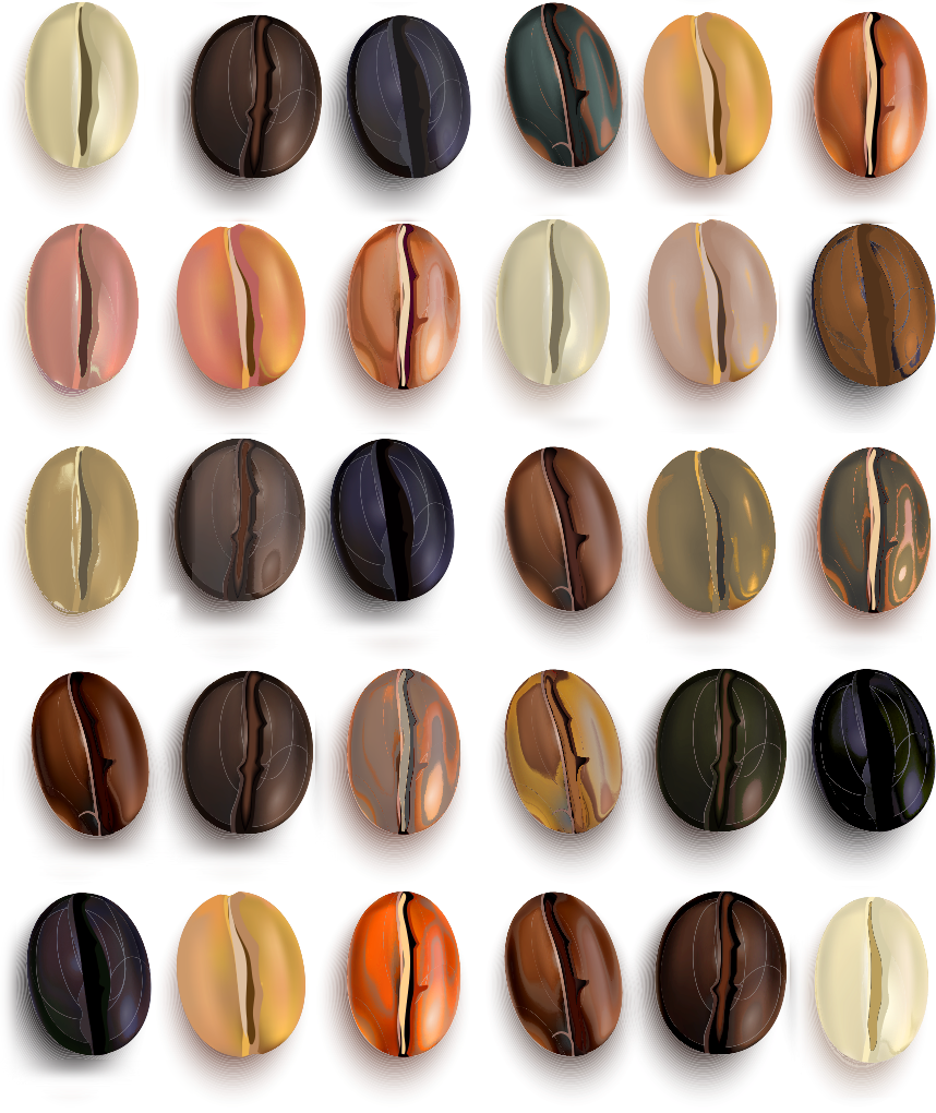
Des grains de café disposés en lignes et colonnes.

Échantillon

Des grains de café en lignes et colonnes, dont la plupart sont grisés.

Échantillonnage aléatoire simple avec remise

Population

Des grains de café disposés en lignes et colonnes.

Échantillon

Un échantillon aléatoire de grains de café, dont certains en double.

Pourquoi échantillonner avec remise ?

Considérez les données coffee_ratings comme un échantillon d'une population plus large de cafés.
Considérez chaque café de notre échantillon comme représentant de nombreux cafés absents de l'échantillon mais présents dans la population.
L'échantillonnage avec remise sert de proxy pour inclure différents membres de ces groupes dans l'échantillon.

Préparation des données café

coffee_focus <- coffee_ratings %>%
  select(variety, country_of_origin, flavor) %>%
  rowid_to_column()

glimpse(coffee_focus)

Rows: 1,338
Columns: 4
$ rowid             <int> 1, 2, 3, 4, 5, 6, 7, 8, 9, 10, 11, 12, 13, 14, 15, ...
$ variety           <chr> NA, "Other", "Bourbon", NA, "Other", NA, "Other", N...
$ country_of_origin <chr> "Ethiopia", "Ethiopia", "Guatemala", "Ethiopia", "E...
$ flavor            <dbl> 8.83, 8.67, 8.50, 8.58, 8.50, 8.42, 8.50, 8.33, 8.6...

Rééchantillonner avec slice_sample()

coffee_resamp <- coffee_focus %>%
  slice_sample(prop = 1, replace = TRUE)

# A tibble: 1,338 x 4
   rowid variety country_of_origin flavor
   <int> <chr>   <chr>              <dbl>
 1  1253 Bourbon Guatemala           6.92
 2   186 Caturra Colombia            7.58
 3  1185 Bourbon Guatemala           7.42
 4  1273 NA      Philippines         6.5 
 5  1042 Caturra Honduras            7.33
 6   195 Caturra Guatemala           7.75
 7  1219 Typica  Mexico              7   
 8   952 Caturra Honduras            7.5 
 9    41 Caturra Thailand            8.33
10   460 Caturra Honduras            7.67
# ... with 1,328 more rows

Cafés répétés

coffee_resamp %>% 
  count(rowid, sort = TRUE)

# A tibble: 844 x 2
   rowid     n
   <int> <int>
 1   704     5
 2   913     5
 3  1070     5
 4    16     4
 5   180     4
 6   230     4
 7   234     4
 8   342     4
 9   354     4
10   423     4
# ... with 834 more rows

Cafés manquants

coffee_resamp %>% 
  summarize(
    coffees_included = n_distinct(rowid),
    coffees_not_included = n() - coffees_included
  )

# A tibble: 1 x 2
  coffees_included coffees_not_included
             <int>                <int>
1              844                  494

Bootstrap

L'inverse de l'échantillonnage à partir d'une population.

Échantillonnage : passer d'une population à un échantillon plus petit.

Bootstrap : construire une population théorique à partir de votre échantillon.

Cas d'usage du bootstrap

Comprendre la variabilité d'échantillonnage à partir d'un seul échantillon.

Une botte de cowboy.

Processus de bootstrap

Créer un rééchantillon de même taille que l'échantillon initial.
Calculer la statistique d'intérêt pour cet échantillon bootstrap.
Répéter les étapes 1 et 2 de nombreuses fois.

Les statistiques obtenues sont des statistiques bootstrap et, vues pour leur variabilité, forment une distribution bootstrap.

Bootstrap de la saveur moyenne du café

# Étape 3. Répéter de nombreuses fois
mean_flavors_1000 <- replicate(
  n = 1000,
  expr = {

    coffee_focus %>%
      # Étape 1. Rééchantillonner
      slice_sample(prop = 1, replace = TRUE) %>%

      # Étape 2. Calculer la statistique
      summarize(mean_flavor = mean(flavor, na.rm = TRUE)) %>% 
      pull(mean_flavor)

})

Histogramme de la distribution bootstrap

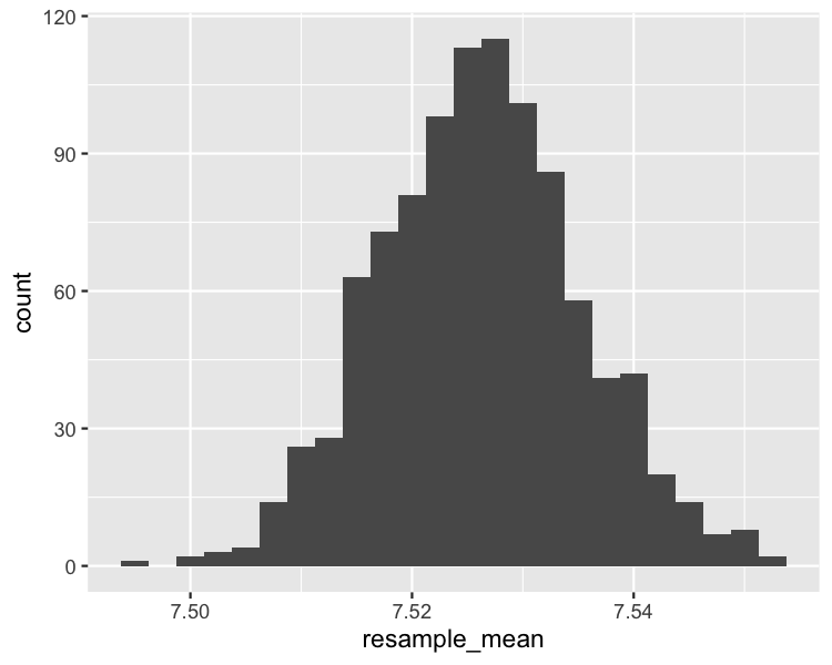
bootstrap_distn <- tibble(
  resample_mean = mean_flavors_1000
)

ggplot(bootstrap_distn, aes(resample_mean)) +
  geom_histogram(binwidth = 0.0025)

Un histogramme de la distribution bootstrap de la moyenne d'échantillon.

Passons à la pratique !