Sélection des variables selon l'AUC

Modélisation du risque de crédit en R

Lore Dirick

Manager of Data Science Curriculum at Flatiron School

Courbes ROC pour 4 modèles de régression logistique

Capture d'écran du 22-06-2020 à 18.31.53.png

Courbes ROC pour 4 modèles de régression logistique

Capture d'écran du 22-06-2020 à 18.31.44.png

Courbes ROC pour 4 modèles de régression logistique

Capture d'écran du 22-06-2020 à 18.31.33.png

Élagage basé sur l'AUC

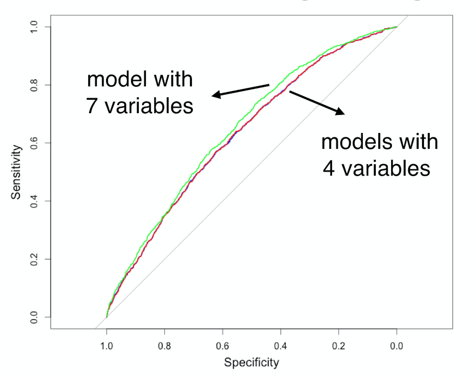
1) Commencez par un modèle incluant toutes les variables (ici, 7) et calculez l'AUC

log_model_full <- glm(loan_status ~ loan_amnt + grade + home_ownership + 
                      annual_inc + age + emp_cat + ir_cat, 
                      family = "binomial", data = training_set)

predictions_model_full <- predict(log_model_full, 
                                  newdata = test_set, type ="response")

AUC_model_full <- auc(test_set$loan_status, predictions_model_full)

Area under the curve: 0.6512

2) Créez 7 nouveaux modèles en retirant à chaque fois une variable, puis faites des prédictions PD sur l'ensemble de test

log_1_remove_amnt <- glm(loan_status ~ grade + home_ownership + annual_inc + age + emp_cat + ir_cat,
                         family = "binomial",
                         data = training_set)

log_1_remove_grade <- glm(loan_status ~ loan_amnt + home_ownership + annual_inc + age + emp_cat + ir_cat,
                          family = "binomial",
                          data = training_set)

log_1_remove_home <- glm(loan_status ~ loan_amnt + grade + annual_inc + age + emp_cat + ir_cat,
                         family = "binomial",
                         data = training_set)

pred_1_remove_amnt <- predict(log_1_remove_amnt, newdata = test_set, type = "response")
pred_1_remove_grade <- predict(log_1_remove_grade, newdata = test_set, type = "response")
pred_1_remove_home <- predict(log_1_remove_home, newdata = test_set, type = "response")
...

3) Conservez le modèle avec la meilleure AUC (AUC du modèle complet : 0,6512)

auc(test_set$loan_status, pred_1_remove_amnt)

Area under the curve: 0.6537

auc(test_set$loan_status, pred_1_remove_grade)

Area under the curve: 0.6438

auc(test_set$loan_status, pred_1_remove_home)

Area under the curve: 0.6537

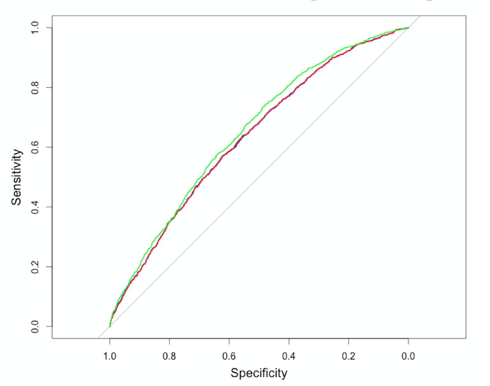
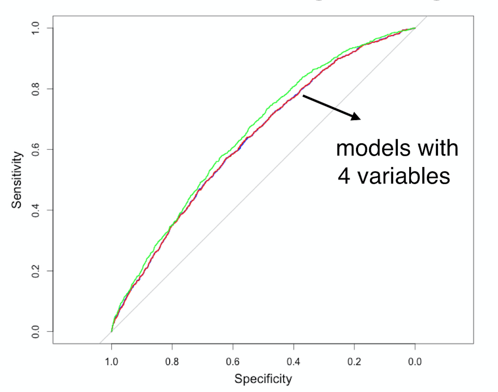
4) Répétez jusqu'à ce que l'AUC diminue (significativement)

Passons à la pratique !

Modélisation du risque de crédit en R