Gérer les données manquantes avec des imputations en R
Michal Oleszak
Machine Learning Engineer

Dans presque la moitié des études, les résultats clés disparaissent
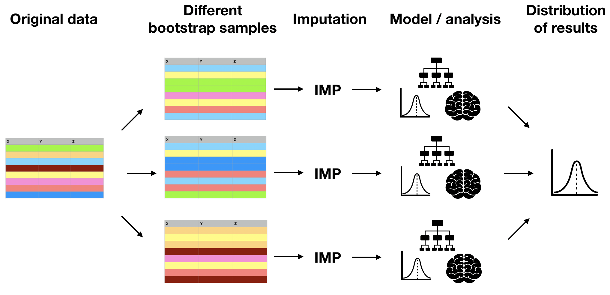
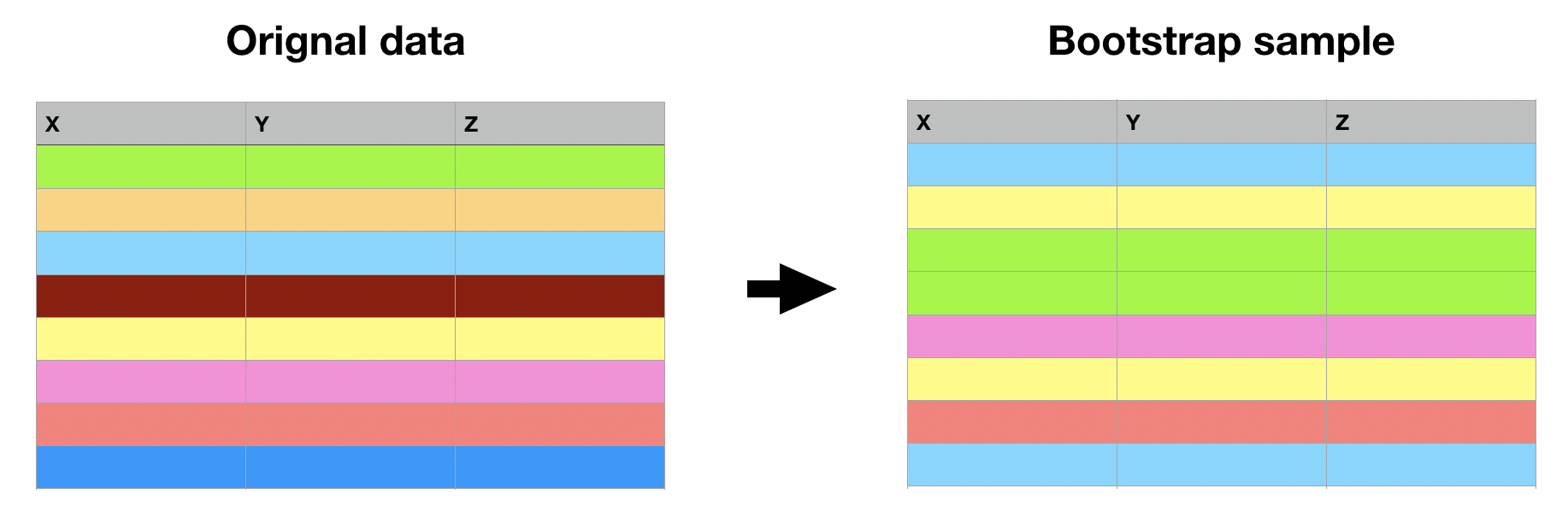
Bootstrap = échantillonner des lignes avec remise pour obtenir une taille d'origine

Avantages :
Limites :
calc_correlation <- function(data, indices) {
# Return the correlation coefficient
return(corr_coeff)
}
calc_correlation <- function(data, indices) {
# Get bootstrap sample
data_boot <- data[indices, ]
# Return the correlation coefficient
return(corr_coeff)
}
calc_correlation <- function(data, indices) {
# Get bootstrap sample
data_boot <- data[indices, ]
# Impute with kNN imputation
data_imp <- kNN(data_boot)
# Return the correlation coefficient
return(corr_coeff)
}
calc_correlation <- function(data, indices) {
# Get bootstrap sample
data_boot <- data[indices, ]
# Impute with kNN imputation
data_imp <- kNN(data_boot)
# Calculate correlation between Weight and TotChol
corr_coeff <- cor(data_imp$Weight, data_imp$TotChol)
# Return the correlation coefficient
return(corr_coeff)
}
library(boot)
boot_results <- boot(nhanes, statistic = calc_correlation, R = 50)
print(boot_results)
BOOTSTRAP NON PARAMÉTRIQUE ORDINAIRE
Appel :
boot(data = nhanes, statistic = calc_correlation, R = 50)
Statistiques du bootstrap :
original biais écart-type
t1* 0.03028306 0.007385452 0.04207152
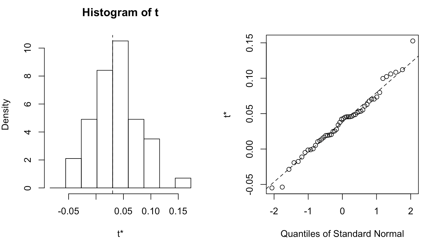
plot(boot_results)

boot_ci <- boot.ci(boot_results, conf = 0.95, type = "norm")
print(boot_ci)
CALCUL DES INTERVALLES DE CONFIANCE PAR BOOTSTRAP
Basé sur 50 réplicas bootstrap
APPEL :
boot.ci(boot.out = boot_results, conf = 0.95, type = "norm")
Intervalles :
Niveau Normal
95% (-0.0596, 0.1054 )
Calculs et intervalles sur l'échelle d'origine
Gérer les données manquantes avec des imputations en R