Lösung: Simulationstest

Supply Chain Analytics mit Python

Aaren Stubberfield

Supply Chain Analytics Mgr.

Achtung

Probleme mit langer Laufzeit solltest du nicht mit LP oder IP lösen

Vorsicht, rutschender Mann

Gesamtkonzept

Grundidee:

Füge ausgewählten Eingaben Zufallsrauschen hinzu
Löse das Modell wiederholt
Beobachte die Verteilung

Warum ausprobieren?

Warum:

Eingaben sind oft Schätzwerte und können ungenau sein.
Frühere Sensitivitätsanalyse änderte jeweils nur eine Eingabe.

Kontext

Kontext – Glasfirma – Ressourcenplanung:

Ressource	Prod. A	Prod. B	Prod. C
Profit $US	$500	$450	$600

Nebenbedingungen:

Es gibt Beschränkungen für Nachfrage, Produktionskapazität und Lagerkapazität

Risiken:

Gewinnschätzungen können ungenau sein

# Initialize Class, & Define Variables
model = LpProblem("Max Glass Co. Profits", LpMaximize)
A = LpVariable('A', lowBound=0)
B = LpVariable('B', lowBound=0)
C = LpVariable('C', lowBound=0)

# Define Objective Function
model += 500 * A + 450 * B + 600 * C

# Define Constraints & Solve
model += 6 * A + 5 * B + 8 * C <= 60
model += 10.5 * A + 20 * B + 10 * C <= 150
model += A  <= 8
model.solve()

Codebeispiel – Schritt 2

a, b, c = normalvariate(0,25), 
          normalvariate(0,25),
          normalvariate(0,25)

# Define Objective Function
model += (500+a)*A + (450+b)*B + (600+c)*C

# Initialize Class, & Define Variables
model = LpProblem("Max Glass Co. Profits", 
                   LpMaximize)

A = LpVariable('A', lowBound=0)
B = LpVariable('B', lowBound=0)
C = LpVariable('C', lowBound=0)
a, b, c = normalvariate(0,25), 
          normalvariate(0,25), 
          normalvariate(0,25)
# Define Objective Function
model += (500+a)*A + (450+b)*B + (600+c)*C

# Define Constraints & Solve
model += 6 * A + 5 * B + 8 * C <= 60
model += 10.5 * A + 20 * B + 10 * C <= 150
model += A  <= 8
model.solve()

def run_pulp_model():
    # Initialize Class
    model = LpProblem("Max Glass Co. Profits", LpMaximize)
    A = LpVariable('A', lowBound=0)
    B = LpVariable('B', lowBound=0)
    C = LpVariable('C', lowBound=0)
    a, b, c = normalvariate(0,25), normalvariate(0,25), normalvariate(0,25)

    # Define Objective Function
    model += (500+a)*A + (450+b)*B + (600+c)*C

    # Define Constraints & Solve
    model += 6 * A + 5 * B + 8 * C <= 60
    model += 10.5 * A + 20 * B + 10 * C <= 150
    model += A  <= 8
    model.solve()
    o = {'A':A.varValue, 'B':B.varValue, 'C':C.varValue, 'Obj':value(model.objective)}
    return(o)

Codebeispiel – Schritt 4

def run_pulp_model():
    # Initialize Class
    model = LpProblem("Max Glass Co. Profits",
                       LpMaximize)
    A = LpVariable('A', lowBound=0)
    B = LpVariable('B', lowBound=0)
    C = LpVariable('C', lowBound=0)
    a, b, c = normalvariate(0,25), 
              normalvariate(0,25),
              normalvariate(0,25)

    # Define Objective Function
    model += (500+a)*A + (450+b)*B + 
             (600+c)*C

    # Define Constraints & Solve
    model += 6 * A + 5 * B + 8 * C <= 60
    model += 10.5 * A + 20 * B + 10 * C <= 150
    model += A  <= 8
    model.solve()
    o = {'A':A.varValue, 'B':B.varValue, 
         'C':C.varValue, 
         'Obj':value(model.objective)}
    return(o)

for i in range(100):
    output.append(run_pulp_model())
df = pd.DataFrame(output)

Codebeispiel – Schritt 5

print(df['A'].value_counts())
print(df['B'].value_counts())
print(df['C'].value_counts())

Ausgabe: (Ergebnisse können variieren)

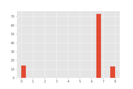
6.666667    73
0.000000    14
8.000000    13
Name: A, dtype: int64

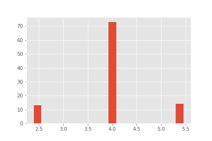
4.000000    73
5.454546    14
2.400000    13
Name: B, dtype: int64
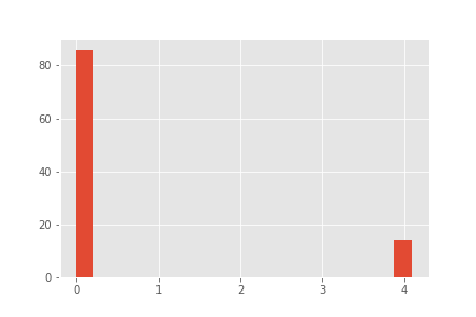
0.000000    86
4.090909    14
Name: C, dtype: int64

Als Histogramm visualisieren

Produkt A: Histogramm zu Produkt A, B, C und Zielwert

Produkt B: Histogramm zu Produkt B

Produkt C: Histogramm zu Produkt C

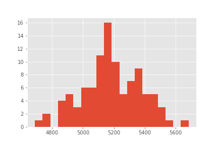
Zielfunktionswerte: Histogramm der Zielfunktionswerte

Zusammenfassung

Nicht für Probleme mit langer Laufzeit verwenden
Vorteile
- Zeigt, wie sich Optima ändern, wenn Eingaben variieren
Schritte
1. Starte mit Standardcode für PuLP-Modelle
2. Füge mit Pythons normalvariate Rauschen zu Schlüsselinformationen hinzu
3. Kapsle den PuLP-Code in eine Funktion, die die Modellausgabe zurückgibt
4. Erstelle eine Schleife, rufe die neue Funktion auf und speichere Ergebnisse im DataFrame
5. Visualisiere den Ergebnis-DataFrame

Probier es aus!

Supply Chain Analytics mit Python