Ohne Fleiß kein Preis

GARCH-Modelle in R

Kris Boudt

Professor of finance and econometrics

GARCH-in-Mean-Modell

Quantifiziere das Risiko-Rendite-Verhältnis.
Risiko: $\sigma^2_t$. Rendite: $\mu_t$.
GARCH-in-Mean-Modell:

$$ \mu_{t} = \mu + \lambda \sigma^2_{t} $$

$\lambda > 0$ ist der Risiko/Rendite-Parameter und gibt die Zunahme der erwarteten Rendite pro Einheit Varianzrisiko an.

Wie?

Ändere das Argument mean.model in ugarchspec() von list(armaOrder = c(0, 0)) zu list(armaOrder = c(0, 0), archm = TRUE, archpow = 2):

garchspec <- ugarchspec(
              mean.model = list(armaOrder = c(0, 0)),
              variance.model = list(model = "gjrGARCH"),
              distribution.model = "sstd")

garchspec <- ugarchspec(
               mean.model = list(armaOrder = c(0, 0), archm = TRUE, archpow = 2),
               variance.model = list(model = "gjrGARCH"),
               distribution.model = "sstd")

Anwendung auf tägliche S&P-500-Renditen

Schätzung

garchfit <- ugarchfit(data = sp500ret, spec = garchspec)

Untersuchung der geschätzten Koeffizienten für den Mittelwert

round(coef(garchfit)[1:2], 4)

    mu  archm 
0.0002 1.9950

Prognostizierte durchschnittliche Renditen

$$ \hat{\mu}_{t} = 0.0002 + 1.9950 \hat{\sigma}^2_{t} $$

Zeitreihendiagramm der prognostizierten Renditen

Zeichne sie in R
```
plot(fitted(garchfit))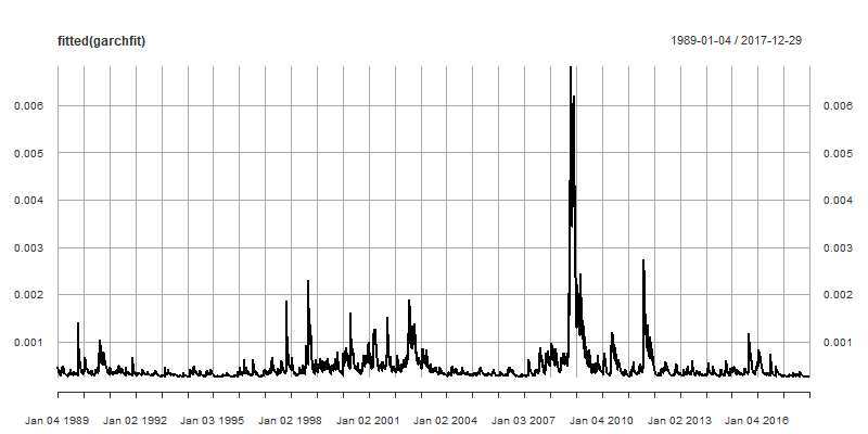
```

Der heutige Return sagt den morgigen voraus

Das GARCH-in-Mean nutzt die finanzielle Theorie des Risiko-Rendite-Abwägung, um ein bedingtes Mittelwertmodell zu bauen.
Jetzt nutzen wir Statistik, um ein Mittelwertmodell zu erstellen, das die Korrelation zwischen heutigem und morgigem Return ausnutzt.
Das populärste Modell ist das AR(1)-Modell:
- AR(1) steht für autoregressives Modell 1. Ordnung.
- Es sagt den nächsten Return über die Abweichung vom langfristigen Mittelwert $\mu$ voraus:

$$ \mu_{t} = \mu + \rho(R_{t-1} - \mu) $$

Ein positiver autoregressiver Koeffizient

$$ \mu_{t} = \mu + \rho(R_{t-1} - \mu) $$

$\rho > 0$:
- Eine über (bzw. unter) dem Durchschnitt liegende Rendite wird von einer über (bzw. unter) dem Durchschnitt liegenden Rendite gefolgt.
- Mögliche Erklärung: Märkte unterreagieren auf Nachrichten, daher Momentum in Renditen.
$|\rho|<1$: Mittelwertumkehr: Die Abweichungen von $R_t$ von $\mu$ sind vorübergehend.

Ein negativer autoregressiver Koeffizient

$$ \mu_{t} = \mu + \rho(R_{t-1} - \mu) $$

$\rho < 0$:
- Eine über (bzw. unter) dem Durchschnitt liegende Rendite wird von einer unter (bzw. über) dem Durchschnitt liegenden Rendite gefolgt.
- Mögliche Erklärung: Märkte überreagieren auf Nachrichten, daher Umkehr in Renditen.

Anwendung auf tägliche S&P-500-Renditen

Spezifikation und Schätzung von AR(1)-GJR-GARCH mit sstd-Verteilung

garchspec <- ugarchspec( 
          mean.model = list(armaOrder = c(1, 0)),
          variance.model = list(model = "gjrGARCH"),
          distribution.model = "sstd")
garchfit <- ugarchfit(data = sp500ret, spec = garchspec)

Schätzer des AR(1)-Modells

round(coef(garchfit)[1:2], 4)

     mu     ar1     
 0.0003 -0.0292

MA(1)- und ARMA(1,1)-Modell

Das gleitende Durchschnittsmodell 1. Ordnung nutzt die Abweichung der Rendite von ihrem bedingten Mittelwert:

$$ \mu_{t} = \mu + \theta(R_{t-1} - \mu_{t-1}) $$

ARMA(1,1) kombiniert AR(1) und MA(1):

$$ \mu_{t} = \mu + \rho(R_{t-1} - \mu) + \theta(R_{t-1} - \mu_{t-1}) $$

Wie?

MA(1)

garchspec <- ugarchspec( 
          mean.model = list(armaOrder = c(0, 1)),
          variance.model = list(model = "gjrGARCH"),
          distribution.model = "sstd")

ARMA(1, 1)

garchspec <- ugarchspec( 
          mean.model = list(armaOrder = c(1, 1)),
          variance.model = list(model = "gjrGARCH"),
          distribution.model = "sstd")

Du bist dran: das Argument mean.model ändern

GARCH-Modelle in R