Avaliando o ajuste do modelo
Modelagem com tidymodels em R

David Svancer
Data Scientist
Classificação binária
Variável de saída com dois níveis
- Classe positiva
- Evento de interesse para prever
- "yes" na variável
purchased
Classe negativa
- "no"
Em
tidymodelsa variável de saída deve ser um fator- O primeiro nível é a classe positiva
- Verifique a ordem com
levels()
leads_df
# A tibble: 1,328 x 7
  purchased total_visits  ...   us_location
   <fct>        <dbl>     ...     <fct>
 1 yes            7       ...     west
 2 no             8       ...     west
 3 no             5       ...     southeast
# ... with 1,325 more rows
levels(leads_df[['purchased']])
[1] "yes" "no"
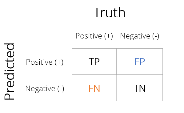
Matriz de confusão
Matriz com contagens de todas as combinações de valores reais e previstos
Previsões corretas
- Verdadeiro positivo (TP)
- Verdadeiro negativo (TN)
Erros de classificação
- Falso positivo (FP)
- Falso negativo (FN)
Métricas de classificação com yardstick
Criando matrizes de confusão e outras métricas de ajuste com yardstick
- Requer um tibble de resultados do modelo contendo:
- Valores reais da saída
purchased
- Categorias previstas
.pred_class
- Probabilidades estimadas de cada categoria
.pred_yes.pred_no
- Valores reais da saída
leads_results
# A tibble: 332 x 4
   purchased .pred_class .pred_yes .pred_no
   <fct>     <fct>           <dbl>    <dbl>
 1 no        no             0.134     0.866
 2 yes       yes            0.729     0.271
 3 no        no             0.133     0.867
 4 no        no             0.0916    0.908
 5 yes       yes            0.598     0.402
 6 no        no             0.128     0.872
 7 yes       no             0.112     0.888
 8 no        no             0.169     0.831
 9 no        no             0.158     0.842
10 yes       yes            0.520     0.480
# ... with 322 more rows
Matriz de confusão com yardstick
A função conf_mat()
- Tibble de resultados do modelo
truth- coluna com os valores reaisestimate- coluna com os valores previstos
Regressão logística em leads_df
- Classificou corretamente 252 de 332 clientes (76%)
- 46 falsos negativos
- 34 falsos positivos
conf_mat(leads_results,truth = purchased,estimate = .pred_class)
Truth
Prediction yes no
yes 74 34
no 46 178
Acurácia da classificação
A função accuracy()
- Recebe os mesmos argumentos de
conf_mat() - Calcula a acurácia da classificação
$$\frac{TP + TN}{TP + TN + FP + FN}$$
- Funções do
yardsticksempre retornam um tibble.metric- tipo de métrica.estimate- valor calculado
accuracy(leads_results,
truth = purchased,
estimate = .pred_class)
# A tibble: 1 x 3
.metric .estimator .estimate
<chr> <chr> <dbl>
1 accuracy binary 0.759
Sensibilidade
Em muitos casos a acurácia não é a melhor métrica
- Dados de
leads_df- Classificar todos como "no" dá 64% de acurácia
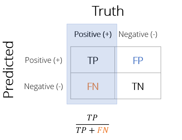
Sensibilidade
Proporção de todos os casos positivos classificados corretamente
- Dos clientes que compraram, que proporção o modelo previu corretamente?
- Menos falsos negativos aumentam a sensibilidade
Calculando a sensibilidade
A função sens()
- Recebe os mesmos argumentos de
conf_mat()eaccuracy() - Retorna a sensibilidade na coluna
.estimate
sens(leads_results,
truth = purchased,
estimate = .pred_class)
# A tibble: 1 x 3
.metric .estimator .estimate
<chr> <chr> <dbl>
1 sens binary 0.617
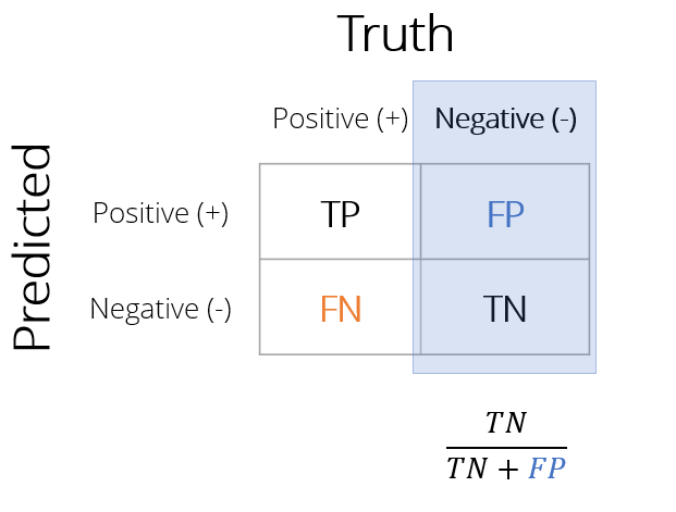
Especificidade
Especificidade é a proporção de todos os casos negativos classificados corretamente
- Dos clientes que não compraram, que proporção o modelo previu corretamente?
- Menos falsos positivos aumentam a especificidade
1 - Especificidade
- Também chamada de taxa de falsos positivos (FPR)
- Proporção de falsos positivos entre os negativos reais
Calculando a especificidade
A função spec()
- Recebe os mesmos argumentos de
sens() - Retorna a especificidade na coluna
.estimate
spec(leads_results,
truth = purchased,
estimate = .pred_class)
# A tibble: 1 x 3
.metric .estimator .estimate
<chr> <chr> <dbl>
1 spec binary 0.840
Criando um conjunto de métricas
Conjuntos de métricas definidos pelo usuário
- Função
metric_set()- Cria uma função personalizada com métricas do
yardstickselecionadas - Passe os nomes das funções do
yardstickemmetric_set() - Use a função personalizada para calcular métricas
- Cria uma função personalizada com métricas do
custom_metrics <-
metric_set(accuracy, sens, spec)
custom_metrics(leads_results,
truth = purchased,
estimate = .pred_class)
# A tibble: 3 x 3
.metric .estimator .estimate
<chr> <chr> <dbl>
1 accuracy binary 0.759
2 sens binary 0.617
3 spec binary 0.840
Muitas métricas
Métricas de classificação binária
Grande variedade de métricas de classificação binária
accuracy(),kap(),sens(),spec(),ppv(),npv(),mcc(),j_index(),bal_accuracy(),detection_prevalence(),precision(),recall(),f_meas()
Passe o resultado de
conf_mat()parasummary()para calcular todas
conf_mat(leads_results,

         truth = purchased,

estimate = .pred_class) %>%
summary()
# A tibble: 13 x 3
   .metric              .estimator .estimate
   <chr>                <chr>          <dbl>
 1 accuracy             binary         0.759
 2 kap                  binary         0.466
 3 sens                 binary         0.617
 4 spec                 binary         0.840
 5 ppv                  binary         0.685
 6 npv                  binary         0.795
 7 mcc                  binary         0.468
 8 j_index              binary         0.456
 9 bal_accuracy         binary         0.728
10 detection_prevalence binary         0.325
11 precision            binary         0.685
12 recall               binary         0.617
13 f_meas               binary         0.649
Vamos praticar!
Modelagem com tidymodels em R

