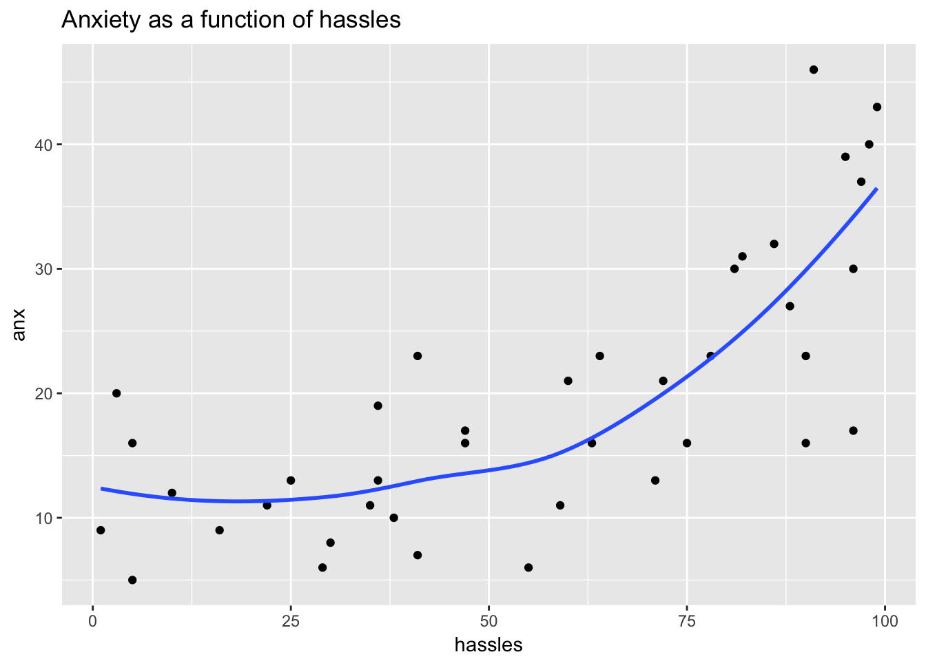
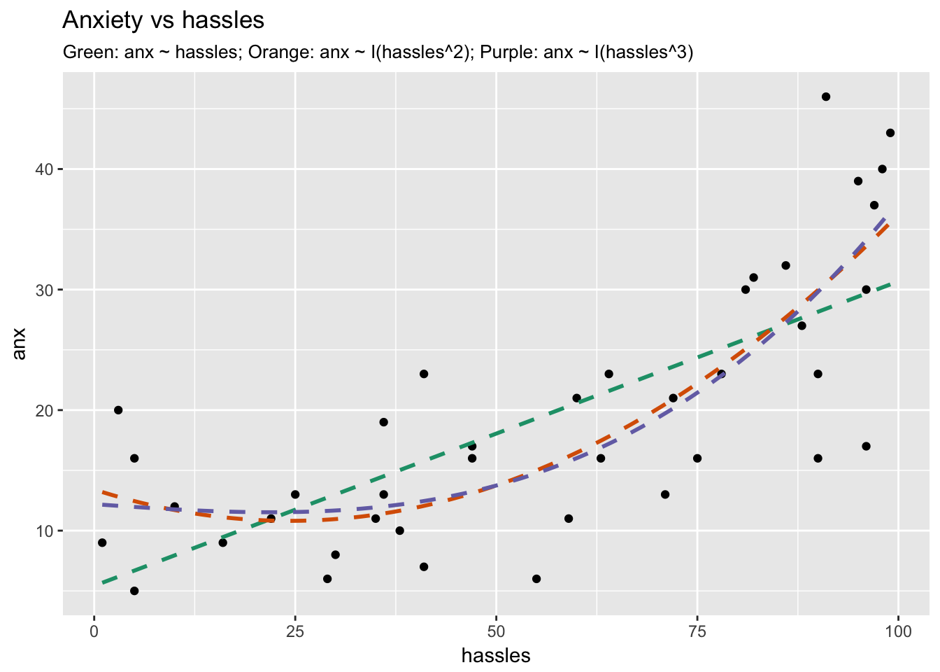
GAM zum Erlernen nichtlinearer Transformationen

Überwachtes Lernen in R: Regression

Nina Zumel and John Mount

Win-Vector, LLC

Generalized Additive Models (GAMs)

$$ y \sim b0 + s1(x1) + s2(x2) + .... $$

Nichtlineare Zusammenhänge lernen

gam() im Paket mgcv

gam(formula, family, data)

family:

gaussian (Standard): „normale" Regression
binomial: Wahrscheinlichkeiten
poisson/quasipoisson: Zählungen

Am besten für größere Datensätze

Die Funktion s()

anx ~ s(hassles)

s() kennzeichnet eine nichtlineare Variable
Verwende s() bei stetigen Variablen
- Mehr als ca. 10 einzigartige Werte

Die hassles-Daten erneut betrachten

Die hassles-Daten erneut betrachten

Modell	RMSE (Cross-Validation)	$R^2$ (Training)
Linear ($hassles$)	7.69	0.53
Quadratisch ($hassles^2$)	6.89	0.63
Kubisch ($hassles^3$)	6.70	0.65

GAM der hassles-Daten

model <- gam(
  anx ~ s(hassles), 
  data = hassleframe, 
  family = gaussian
)

summary(model)

...

R-sq.(adj) =  0.619   Deviance explained = 64.1%
GCV = 49.132  Scale est. = 45.153    n = 40

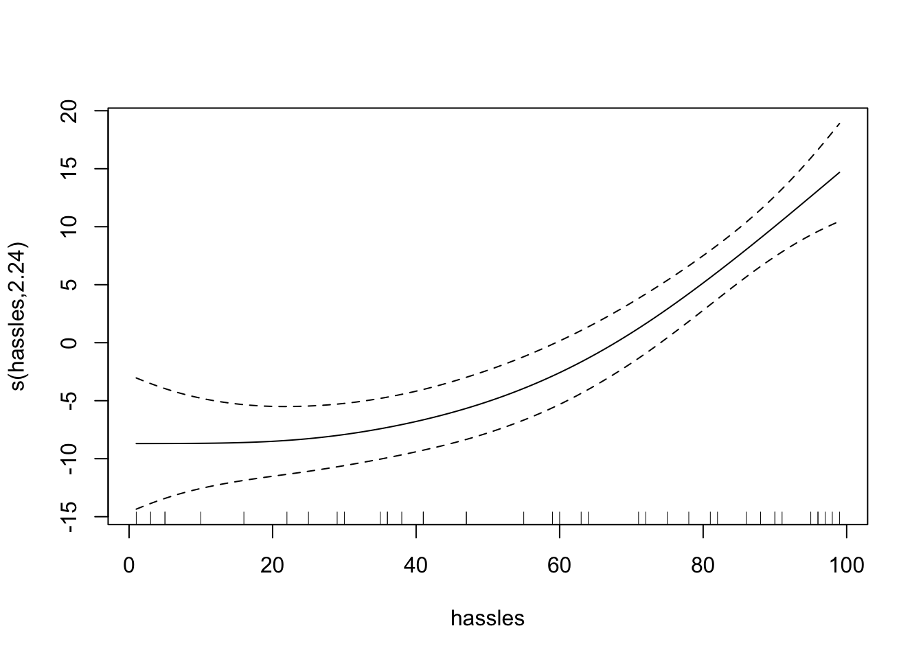
Die Transformationen untersuchen

plot(model)

$y$-Werte: predict(model, type = "terms")

Mit dem Modell vorhersagen

predict(model, newdata = hassleframe, type = "response")

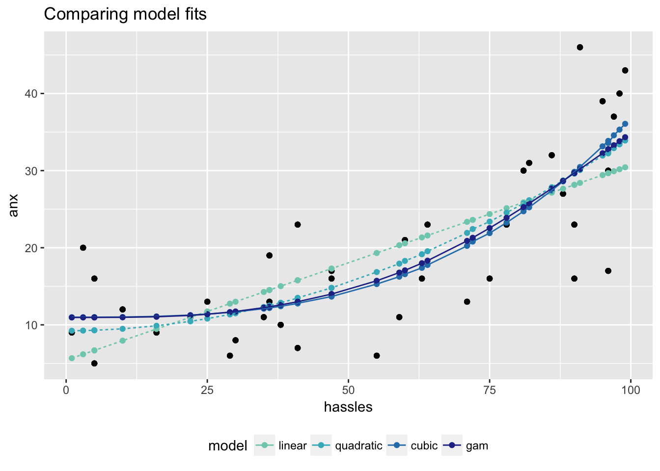
Out-of-Sample-Leistung vergleichen

Die richtige Transformation zu kennen ist ideal, aber GAM hilft, wenn sie unbekannt ist

Modell	RMSE (Cross-Validation)	$R^2$ (Training)
Linear ($hassles$)	7.69	0.53
Quadratisch ($hassles^2$)	6.89	0.63
Kubisch ($hassles^3$)	6.70	0.65
GAM	7.06	0.64

Kleiner Datensatz $\rightarrow$ stärkeres Rauschen im GAM

Lass uns üben!

Überwachtes Lernen in R: Regression

Preparing Video For Download...