Reordenar factores

Datos categóricos en el Tidyverse

Emily Robinson

Data Scientist

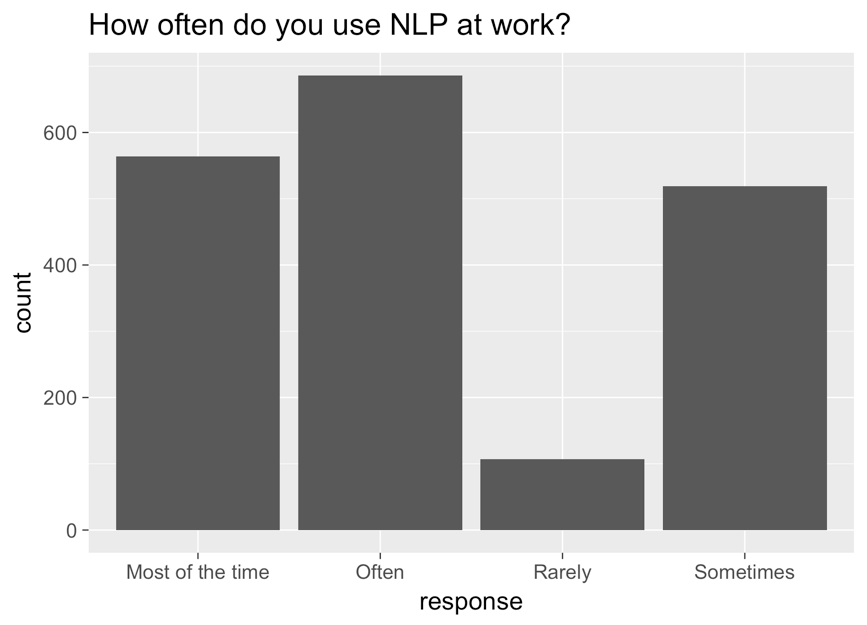
Un diagrama de barras con la variable response en el eje x, count en el eje y y el título «how often do you use NLP at work?». De izquierda a derecha: most of the time, often, rarely y sometimes.

Gráfico corregido

ggplot(aes(nlp_frequency, 
            x = fct_relevel(response, 
            "Rarely", "Sometimes", "Often", "Most of the time"))) + 
        geom_bar()

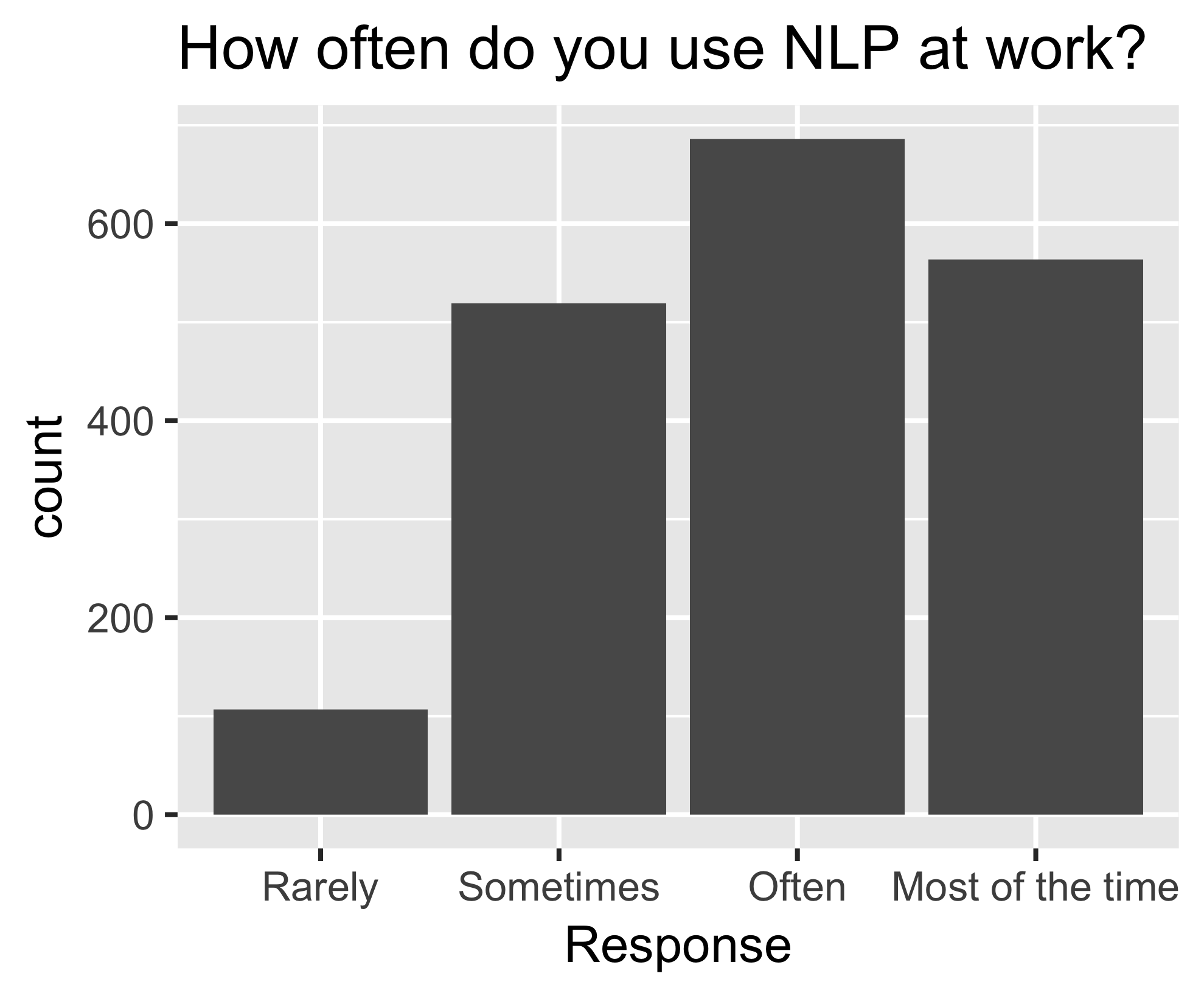
El mismo diagrama de barras que antes, ahora ordenado de izquierda a derecha: rarely, sometimes, often y most of the time.

fct_reorder()

nlp_frequency %>%
    pull(response) %>%
    levels()

[1] "Most of the time" "Often" "Rarely" "Sometimes"

nlp_frequency %>%
    mutate(response = fct_relevel(response, 
            "Often", "Most of the time")) %>%
    pull(response) %>%
    levels()

[1] "Often" "Most of the time" "Rarely" "Sometimes"

Argumentos adicionales

nlp_frequency %>%
    mutate(response = fct_relevel(response, 
            "Often", "Most of the time", after = 2)) %>%
            pull(response) %>%
            levels()

nlp_frequency %>%
    mutate(response = fct_relevel(response, 
            "Often", "Most of the time", after = Inf) %>%
    pull(response) %>%
    levels()

[1] "Rarely" "Sometimes" "Often" "Most of the time"

¡Vamos a practicar!

Datos categóricos en el Tidyverse