Regressão harmônica dinâmica
Previsão em R

Rob J. Hyndman
Professor of Statistics at Monash University
Regressão harmônica dinâmica

Regressão harmônica dinâmica
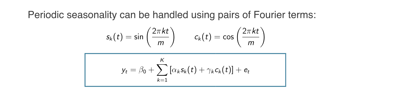
$m =$ período sazonal
Toda função periódica pode ser aproximada por somas de termos sen e cos para K suficientemente grande
Coeficientes de regressão: $\alpha_k$ e $\gamma_k$
$e_t$ pode ser modelado como um processo ARIMA não sazonal
Assume padrão sazonal inalterado
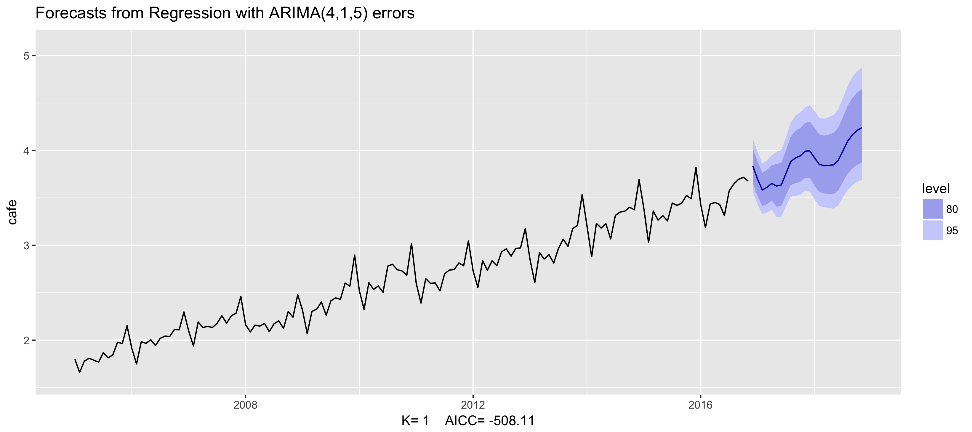
Exemplo: gasto em cafés na Austrália
fit <- auto.arima(cafe, xreg = fourier(cafe, K = 1),
                  seasonal = FALSE, lambda = 0)
fit %>% forecast(xreg = fourier(cafe, K = 1, h = 24)) %>%
   autoplot() + ylim(1.6, 5.1)
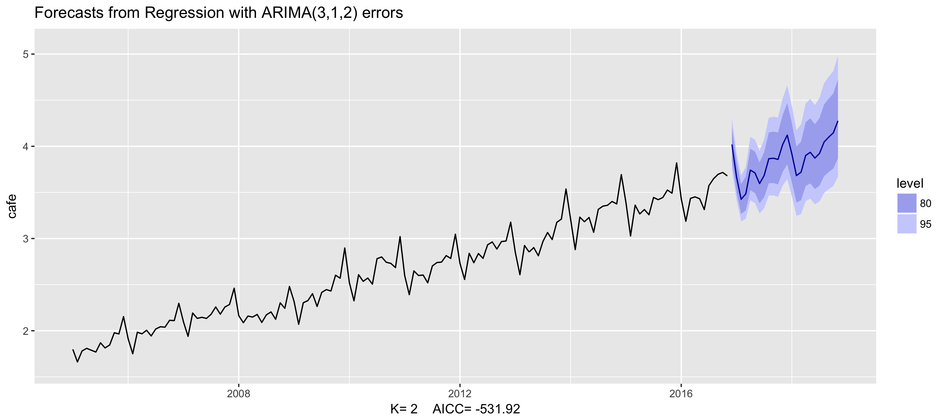
Exemplo: gasto em cafés na Austrália
fit <- auto.arima(cafe, xreg = fourier(cafe, K = 2),
                  seasonal = FALSE, lambda = 0)
fit %>% forecast(xreg = fourier(cafe, K = 2, h = 24)) %>%
   autoplot() + ylim(1.6, 5.1)
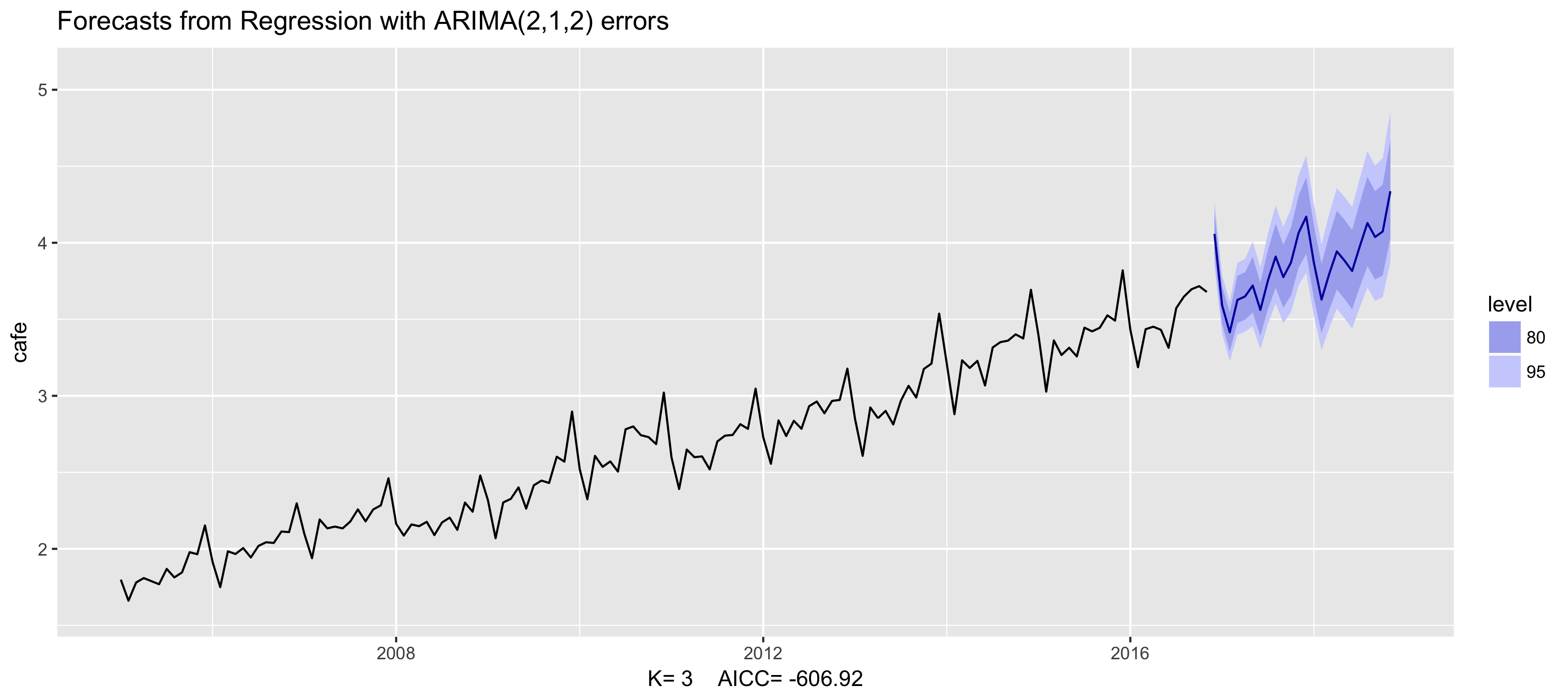
Exemplo: gasto em cafés na Austrália
fit <- auto.arima(cafe, xreg = fourier(cafe, K = 3),
                  seasonal = FALSE, lambda = 0)
fit %>% forecast(xreg = fourier(cafe, K = 3, h = 24)) %>%
   autoplot() + ylim(1.6, 5.1)
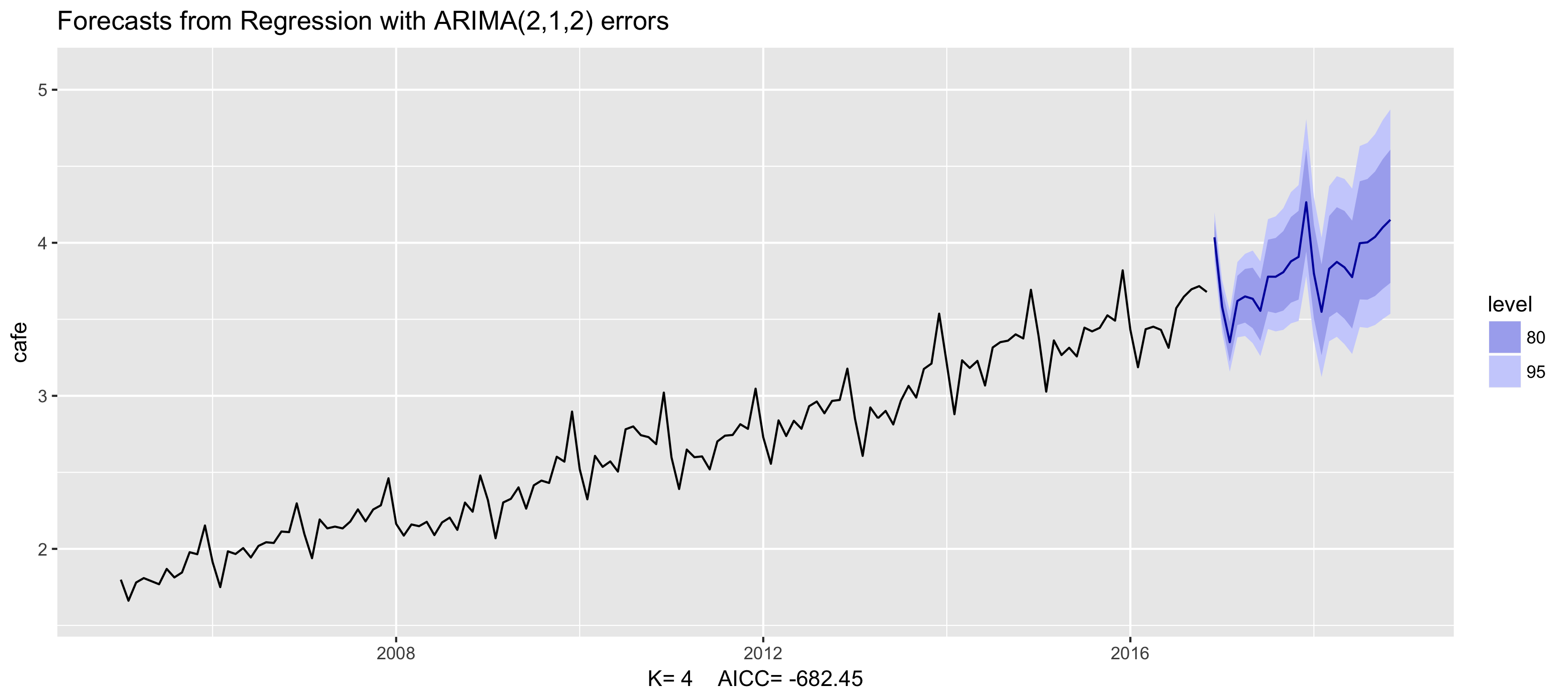
Exemplo: gasto em cafés na Austrália
fit <- auto.arima(cafe, xreg = fourier(cafe, K = 4),
                  seasonal = FALSE, lambda = 0)
fit %>% forecast(xreg = fourier(cafe, K = 4, h = 24)) %>%
   autoplot() + ylim(1.6, 5.1)
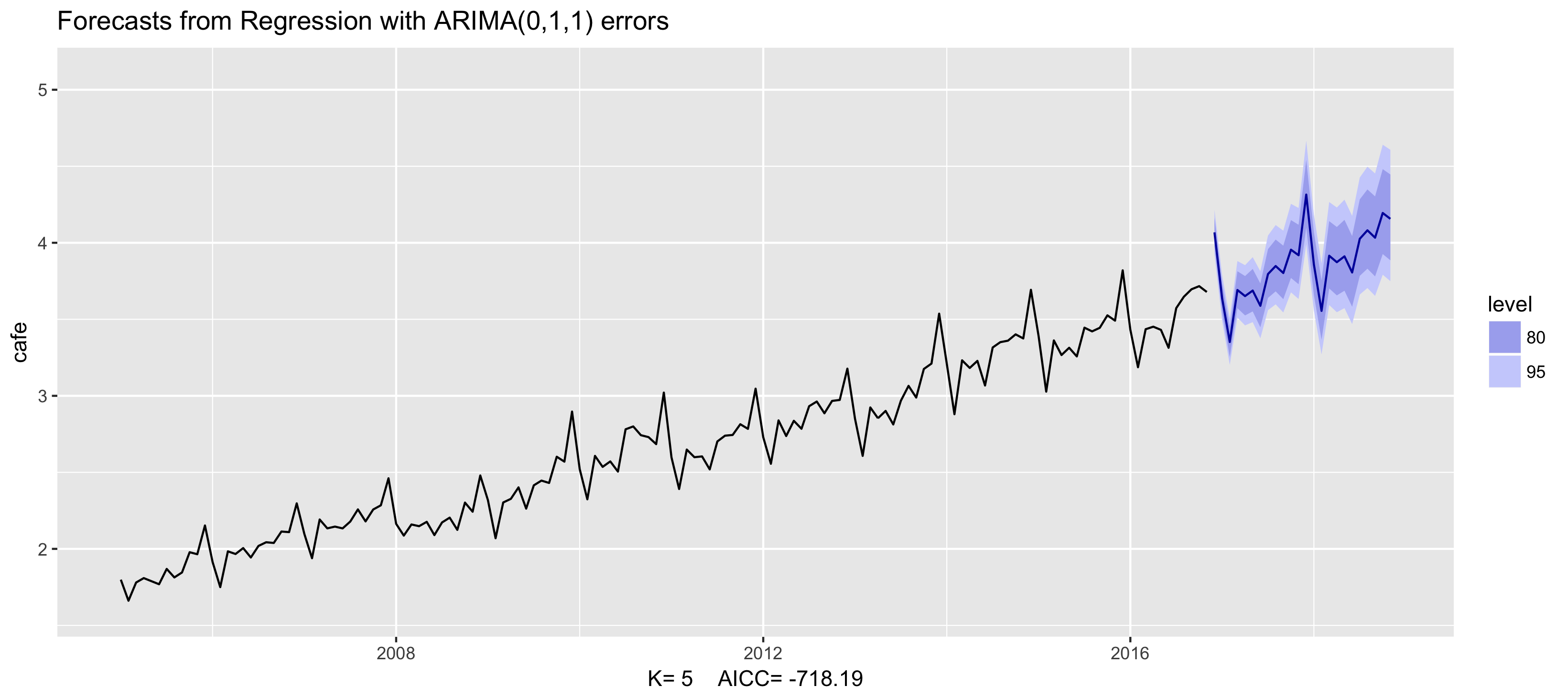
Exemplo: gasto em cafés na Austrália
fit <- auto.arima(cafe, xreg = fourier(cafe, K = 5),
                  seasonal = FALSE, lambda = 0)
fit %>% forecast(xreg = fourier(cafe, K = 5, h = 24)) %>%
   autoplot() + ylim(1.6, 5.1)
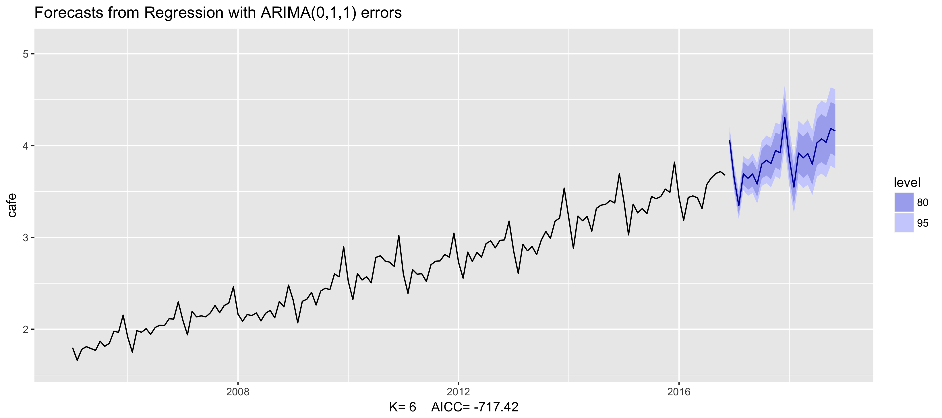
Exemplo: gasto em cafés na Austrália
fit <- auto.arima(cafe, xreg = fourier(cafe, K = 6),
                  seasonal = FALSE, lambda = 0)
fit %>% forecast(xreg = fourier(cafe, K = 6, h = 24)) %>%
   autoplot() + ylim(1.6, 5.1)
Regressão harmônica dinâmica

- Outras variáveis preditoras também podem ser incluídas: $x_{t,1},...,x_{t,r}$
- Escolha K para minimizar o $AIC_c$
- K não pode ser maior que m/2
- Útil especialmente para dados semanais, diários e subdiários.

