Attenzione alla correlazione

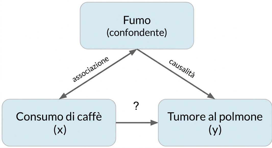
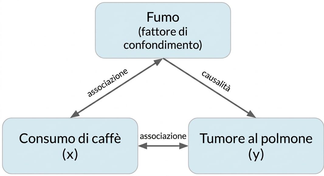
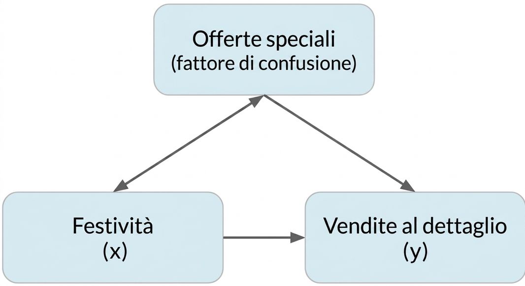
Introduzione alla statistica in Python

Maggie Matsui

Content Developer, DataCamp

Relazioni non lineari

scatterplot di variabili con relazione quadratica

$$r = 0.18$$

Relazioni non lineari

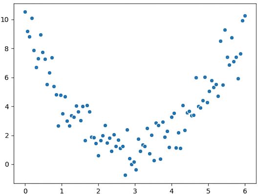
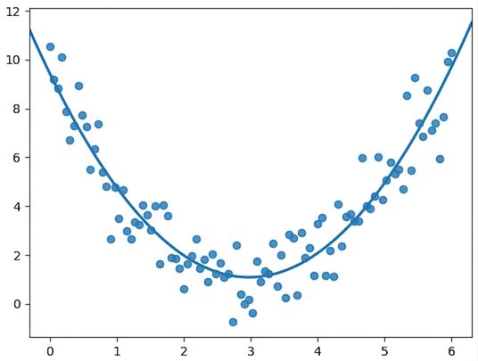
Cosa vediamo:

scatterplot di variabili con relazione quadratica e curva quadratica

Cosa vede il coefficiente di correlazione:

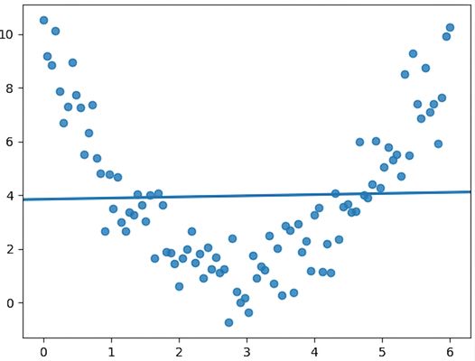
scatterplot di variabili con relazione quadratica e retta lineare

La correlazione copre solo relazioni lineari

Non usare la correlazione alla cieca

df['x'].corr(df['y'])

0.081094

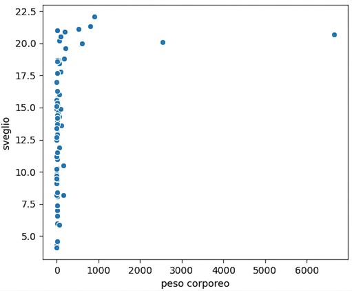
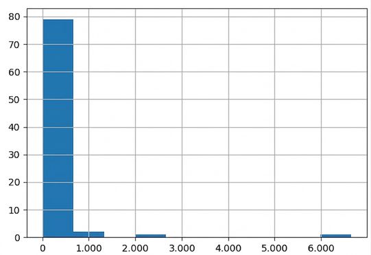
Visualizza sempre i dati

scatterplot di variabili con relazione quadratica

Dati sul sonno dei mammiferi

print(msleep)

                 name       genus   vore         order  ... sleep_cycle  awake  brainwt   bodywt
1             Cheetah    Acinonyx  carni     Carnivora  ...         NaN   11.9      NaN   50.000
2          Owl monkey       Aotus   omni      Primates  ...         NaN    7.0  0.01550    0.480
3     Mountain beaver  Aplodontia  herbi      Rodentia  ...         NaN    9.6      NaN    1.350
4 Greater short-ta...     Blarina   omni  Soricomorpha  ...    0.133333    9.1  0.00029    0.019
5                 Cow         Bos  herbi  Artiodactyla  ...    0.666667   20.0  0.42300  600.000
..                ...         ...    ...           ...  ...         ...    ...      ...      ...
79         Tree shrew      Tupaia   omni    Scandentia  ...    0.233333   15.1  0.00250    0.104
80 Bottle-nosed do...    Tursiops  carni       Cetacea  ...         NaN   18.8      NaN  173.330
81              Genet     Genetta  carni     Carnivora  ...         NaN   17.7  0.01750    2.000
82         Arctic fox      Vulpes  carni     Carnivora  ...         NaN   11.5  0.04450    3.380
83            Red fox      Vulpes  carni     Carnivora  ...    0.350000   14.2  0.05040    4.230

Peso corporeo vs tempo sveglio

Scatterplot di peso corporeo vs tempo sveglio

msleep['bodywt'].corr(msleep['awake'])

0.3119801

Distribuzione del peso corporeo

Istogramma della variabile bodywt

Trasformazione log

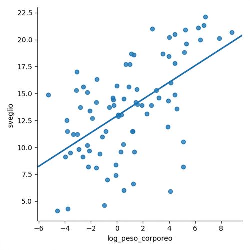
msleep['log_bodywt'] = np.log(msleep['bodywt'])


sns.lmplot(x='log_bodywt',
           y='awake',
           data=msleep,
           ci=None)
plt.show()

msleep['log_bodywt'].corr(msleep['awake'])

0.5687943

Scatterplot di log bodywt vs tempo sveglio

Altre trasformazioni

Trasformazione log (log(x))
Radice quadrata (sqrt(x))
Reciproca (1 / x)
Combinazioni, ad es.:
- log(x) e log(y)
- sqrt(x) e 1 / y

Perché usare una trasformazione?

Alcuni metodi statistici richiedono una relazione lineare
- Coefficiente di correlazione
- Regressione lineare

Introduzione alla modellazione lineare in Python

La correlazione non implica causalità

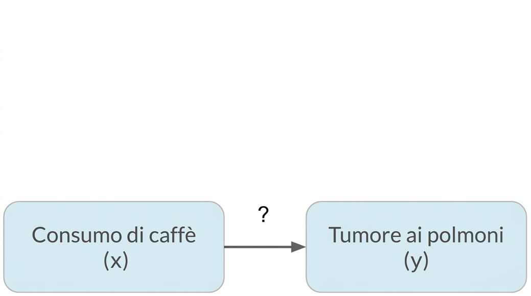
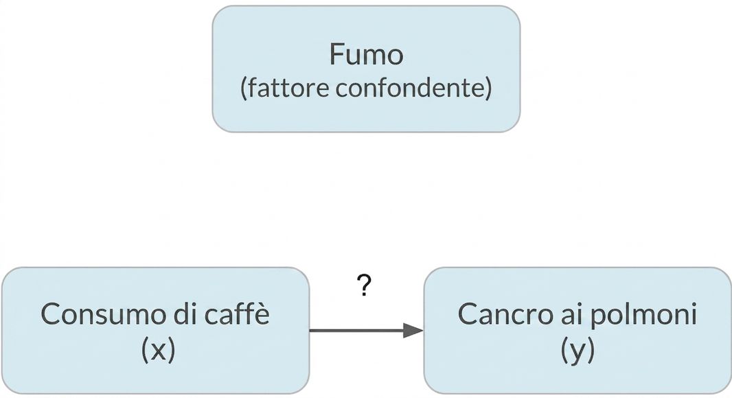
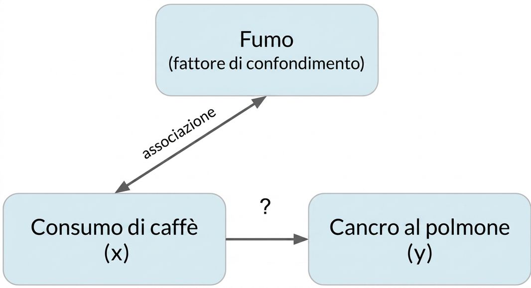
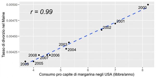
x è correlata con y non significa x causa y

Scatterplot del consumo pro capite di margarina negli USA vs tasso di divorzio nel Maine. Le variabili sono altamente correlate con coefficiente 0,99

Fattori confondenti

Bere caffè (x) che punta a cancro ai polmoni (y)

Fattori confondenti

Bere caffè (x) che punta a cancro ai polmoni (y) con fumo (confondente) sopra

Fattori confondenti

Bere caffè (x) che punta a cancro ai polmoni (y) con fumo (confondente). Doppia freccia tra fumo e caffè, etichetta "associazione".

Fattori confondenti

Bere caffè (x) che punta a cancro ai polmoni (y) con fumo (confondente). Doppia freccia tra fumo e caffè, etichetta "associazione". Freccia da fumo a cancro ai polmoni, etichetta "causalità"

Fattori confondenti

Bere caffè (x) con doppia freccia verso cancro ai polmoni (y) etichettata "associazione". Doppia freccia tra fumo e caffè, "associazione". Freccia da fumo a cancro ai polmoni, "causalità".

Festività (x) punta a vendite retail (y). Offerte speciali (confondente) ha doppia freccia con festività e singola freccia verso vendite retail.

Passons à la pratique !

Introduzione alla statistica in Python