Scatter plots
Introduzione alla visualizzazione dei dati con ggplot2

Rick Scavetta
Founder, Scavetta Academy
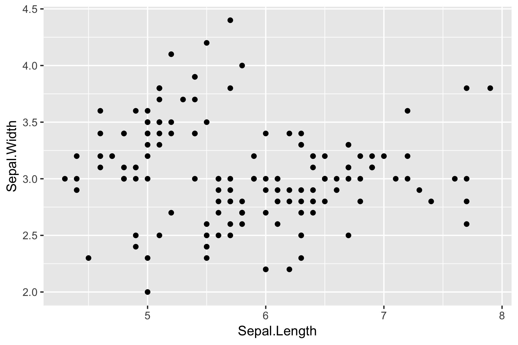
Scatter plots
ggplot(iris, aes(x = Sepal.Length,
                 y = Sepal.Width)) +
  geom_point()
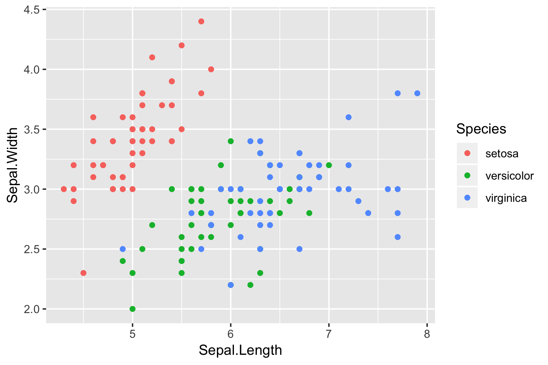
Scatter plots
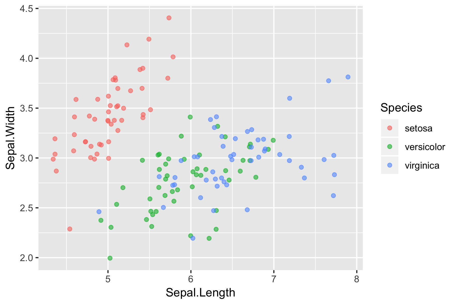
ggplot(iris, aes(x = Sepal.Length,
                 y = Sepal.Width,
                 col = Species)) +
  geom_point()

Geom-specific aesthetic mappings
# These result in the same plot!
ggplot(iris, aes(x = Sepal.Length, y = Sepal.Width, col = Species)) +
  geom_point()

ggplot(iris, aes(x = Sepal.Length, y = Sepal.Width)) +
  geom_point(aes(col = Species))
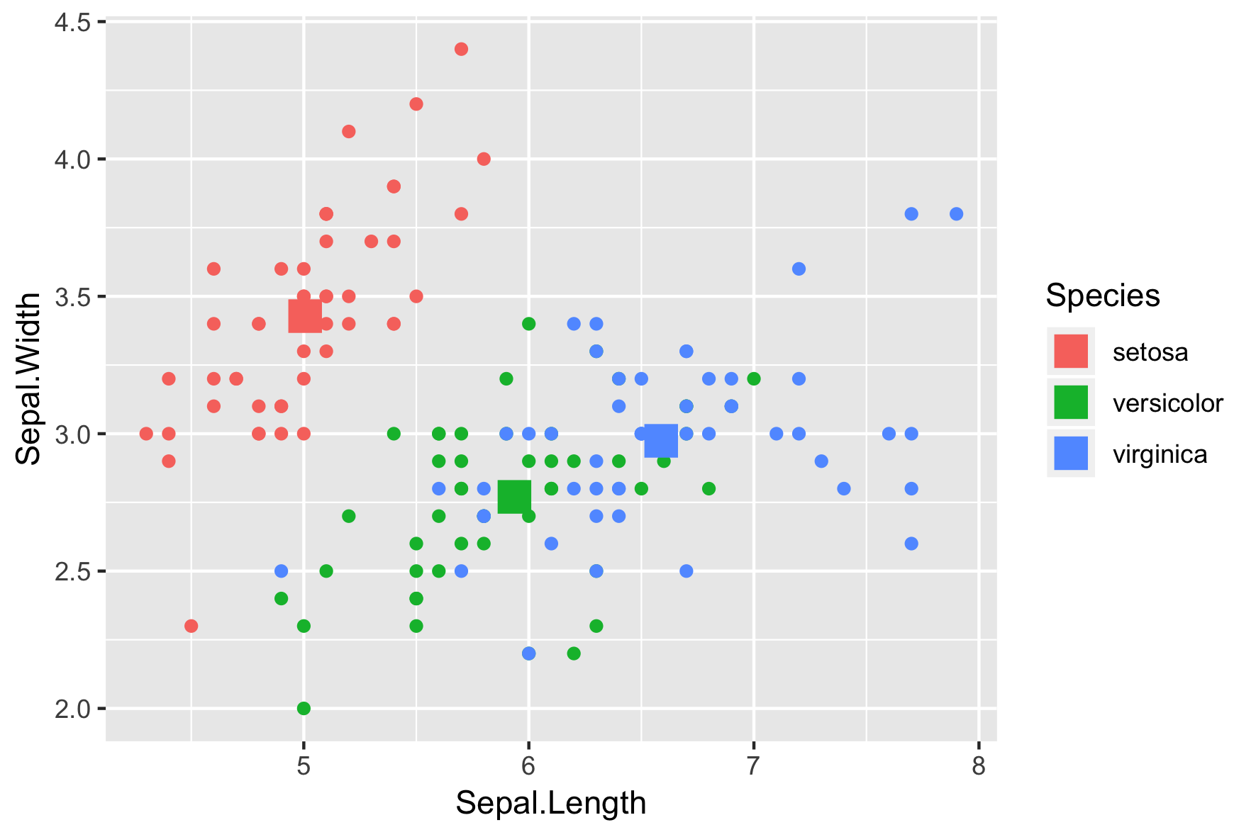
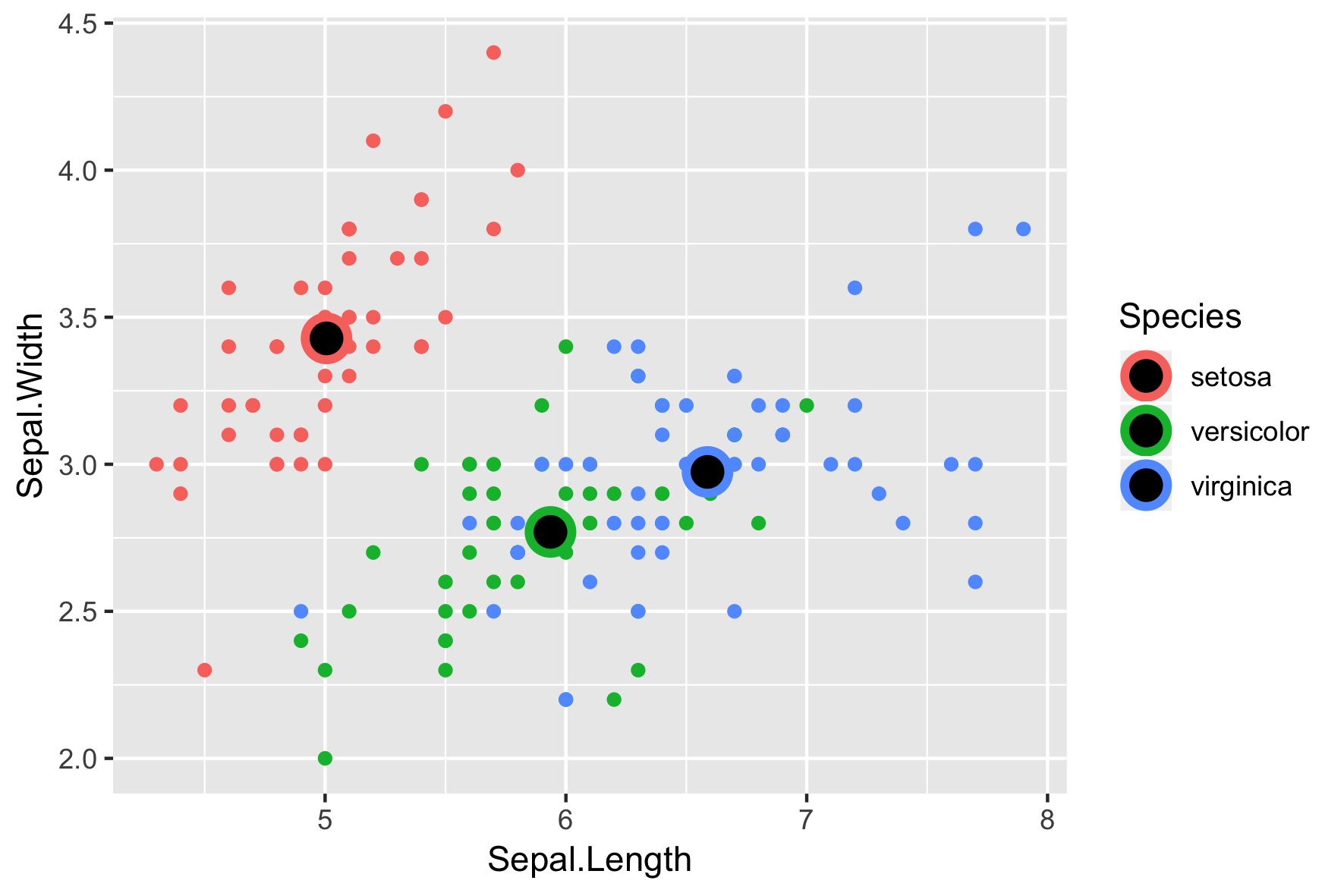
Control aesthetic mappings of each layer independently:
ggplot(iris, aes(x = Sepal.Length, y = Sepal.Width, col = Species)) +
  # Inherits both data and aes from ggplot()
  geom_point() +
  # Different data, but inherited aes
  geom_point(data = iris.summary, shape = 15, size = 5)
Shape attribute values
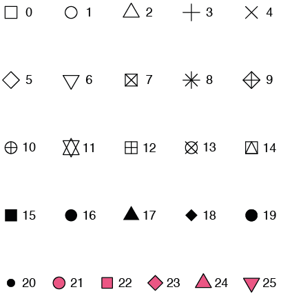
Example
ggplot(iris, aes(x = Sepal.Length, y = Sepal.Width, col = Species)) +
  geom_point() +
  geom_point(data = iris.summary, shape = 21, size = 5,
             fill = "black", stroke = 2)
On-the-fly stats by ggplot2
- See the second course for the stats layer.
- Note: Avoid plotting only the mean without a measure of spread, e.g. the standard deviation.
position = "jitter"
ggplot(iris, aes(x = Sepal.Length, y = Sepal.Width, col = Species)) +
  geom_point(position = "jitter")
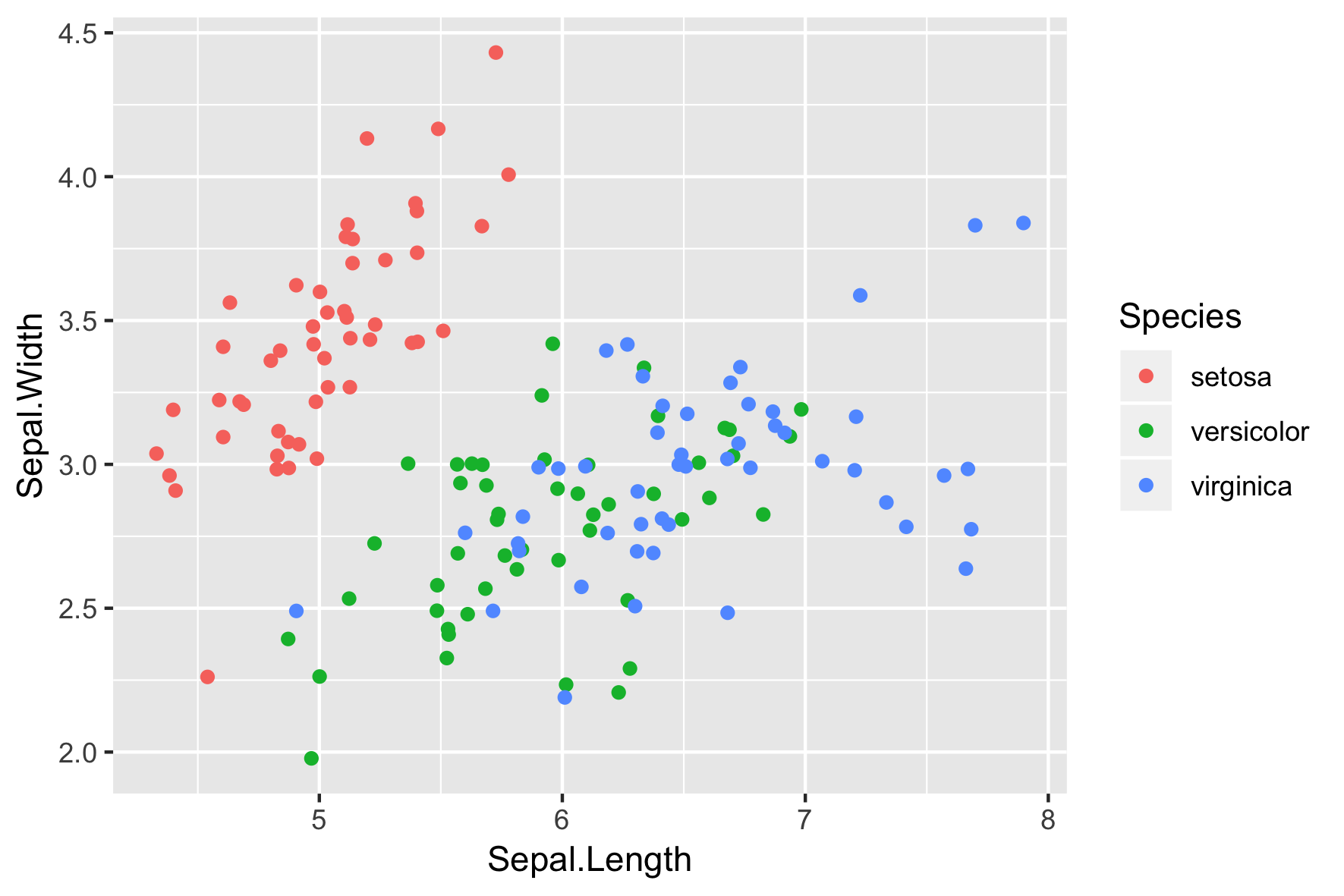
geom_jitter()
A short-cut to geom_point(position = "jitter")
ggplot(iris, aes(x = Sepal.Length, y = Sepal.Width, col = Species)) +
  geom_jitter()
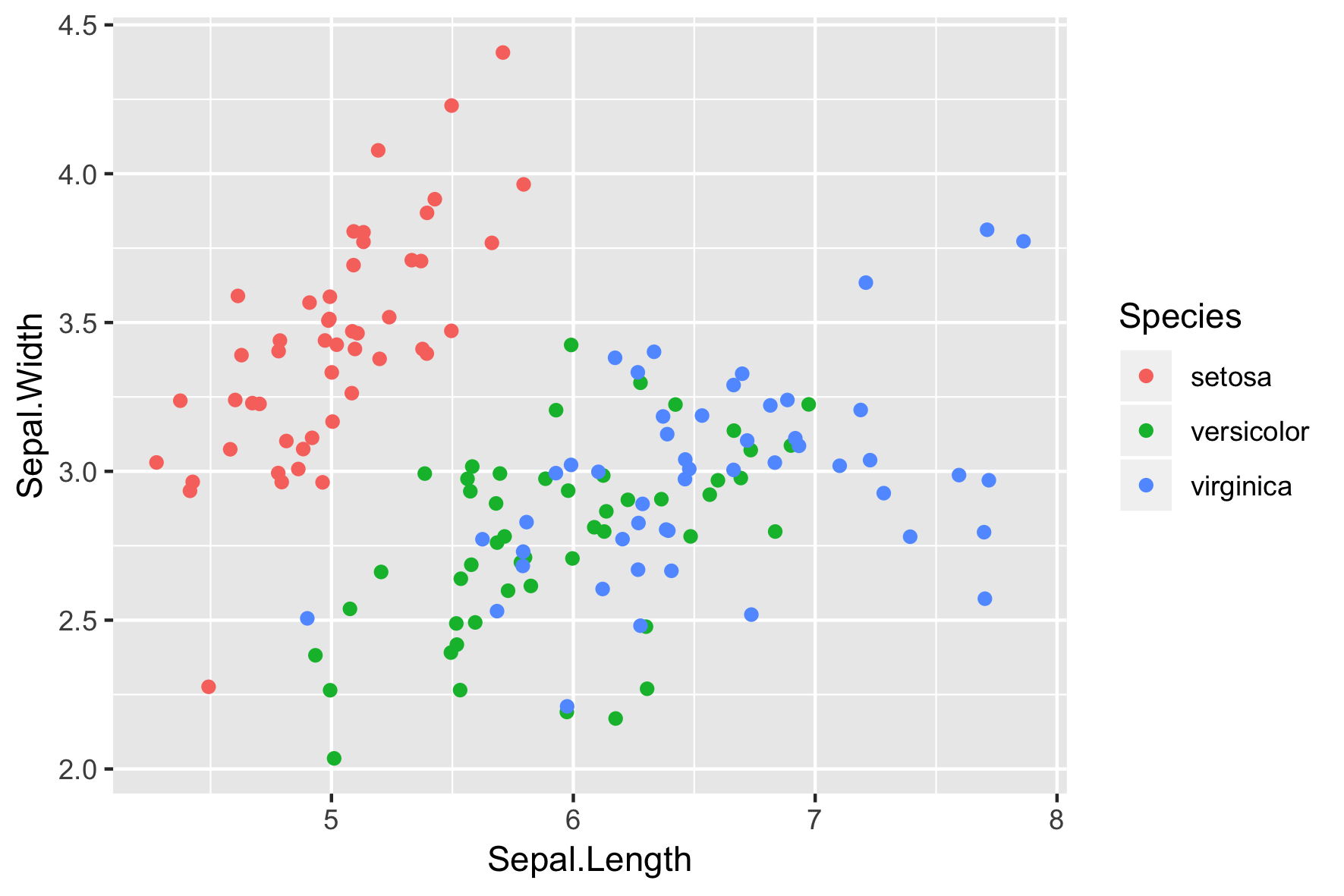
Don't forget to adjust alpha
- Combine jittering with alpha-blending if necessary
ggplot(iris, aes(x = Sepal.Length, y = Sepal.Width, col = Species)) +
  geom_jitter(alpha = 0.6)
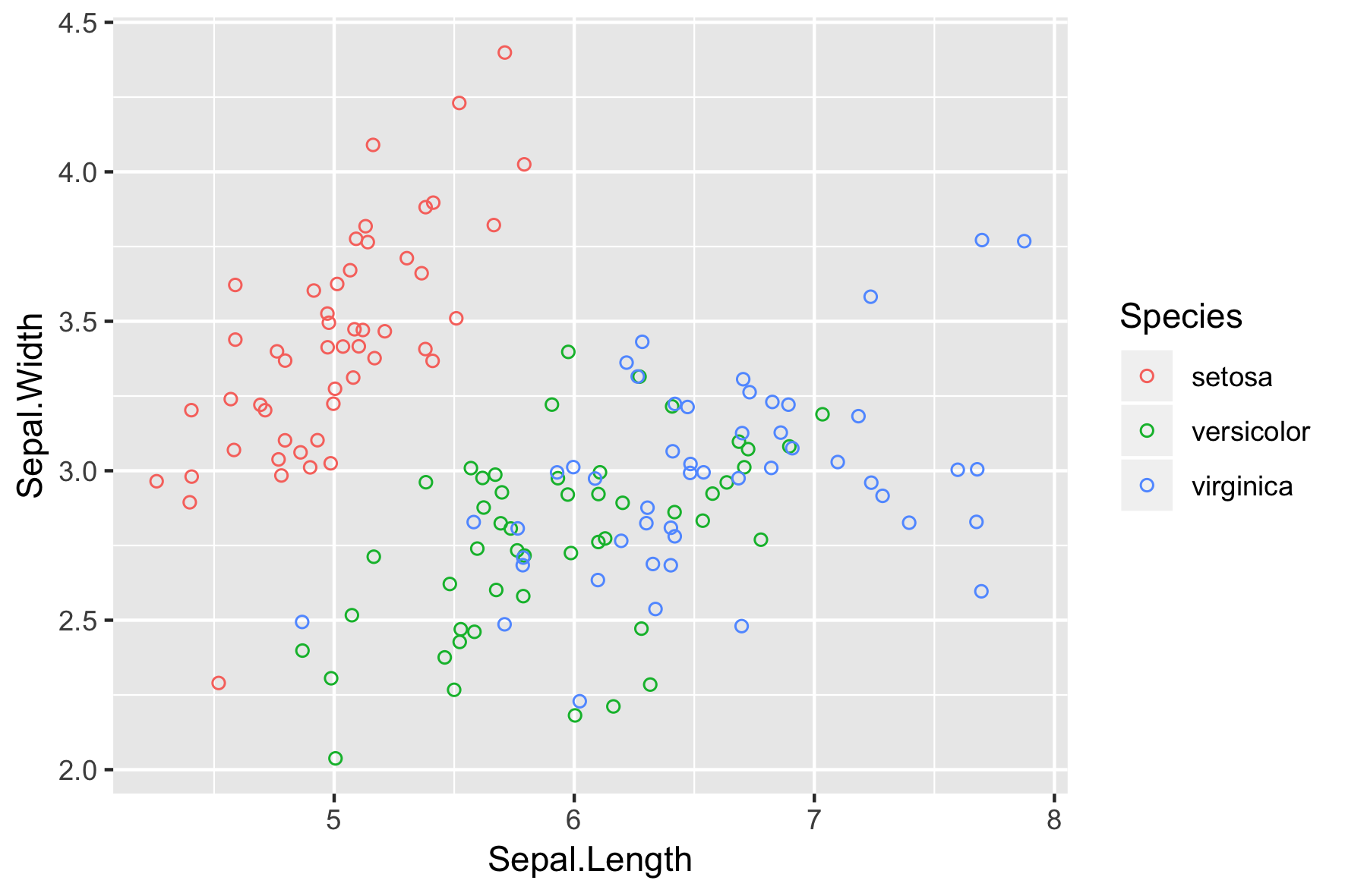
Hollow circles also help
shape = 1is a. hollow circle.- Not necessary to also use alpha-blending.
ggplot(iris, aes(x = Sepal.Length, y = Sepal.Width, col = Species)) +
  geom_jitter(shape = 1)