Transforming variables

Introduzione alla regressione in R

Richie Cotton

Data Evangelist at DataCamp

Perch dataset

library(dplyr)

perch <- fish %>%
  filter(species == "Perch")

species	mass_g	length_cm
Perch	5.9	7.5
Perch	32.0	12.5
Perch	40.0	13.8
Perch	51.5	15.0
Perch	70.0	15.7
...	...	...

It's not a linear relationship

ggplot(perch, aes(length_cm, mass_g)) +
  geom_point() +
  geom_smooth(method = "lm", se = FALSE)

A scatter plot of perch masses versus their lengths, with a trend line. The perches get heavier faster than linearly as they get longer, resulting in an upward curve.

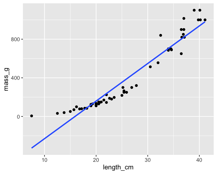
Bream vs. perch

Some bream swimming. Bream are quite flat.

Some perch swimming. Perch are quite round.

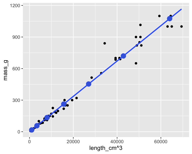
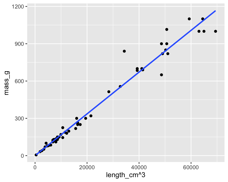
Plotting mass vs. length cubed

ggplot(perch, aes(length_cm ^ 3, mass_g)) +
  geom_point() +
  geom_smooth(method = "lm", se = FALSE)

A scatter plot of perch masses versus their lengths cubed, with a trend line. After this transformation, the points are mostly close to the trend line.

Modeling mass vs. length cubed

mdl_perch <- lm(mass_g ~ I(length_cm ^ 3), data = perch)

Call:
lm(formula = mass_g ~ I(length_cm^3), data = perch)

Coefficients:
   (Intercept)  I(length_cm^3)  
       -0.1175          0.0168

Predicting mass vs. length cubed

explanatory_data <- tibble(
  length_cm = seq(10, 40, 5)
)

prediction_data <- explanatory_data %>%
  mutate(
    mass_g = predict(mdl_perch, explanatory_data)
  )

# A tibble: 7 x 2
  length_cm mass_g
      <dbl>  <dbl>
1        10   16.7
2        15   56.6
3        20  134. 
4        25  262. 
5        30  453. 
6        35  720. 
7        40 1075.

Plotting mass vs. length cubed

ggplot(perch, aes(length_cm ^ 3, mass_g)) +
  geom_point() +
  geom_smooth(method = "lm", se = FALSE) +
  geom_point(data = prediction_data, color = "blue")

The scatter plot of perch masses versus their lengths cubed, with a trend line, annotated with points calculated from the predict() function. The points follow the trend line exactly.

ggplot(perch, aes(length_cm, mass_g)) +
  geom_point() +
  geom_smooth(method = "lm", se = FALSE) +
  geom_point(data = prediction_data, color = "blue")

The scatter plot of perch masses versus their lengths, with a trend line, annotated with points calculated from the predict() function. The points don't follow the trend line but they do follow the curve of the data points.

Facebook advertising dataset

How advertising works

Pay Facebook to shows ads.
People see the ads ("impressions").
Some people who see it, click it.

936 rows
Each row represents 1 advert

spent_usd	n_impressions	n_clicks
1.43	7350	1
1.82	17861	2
1.25	4259	1
1.29	4133	1
4.77	15615	3
...	...	...

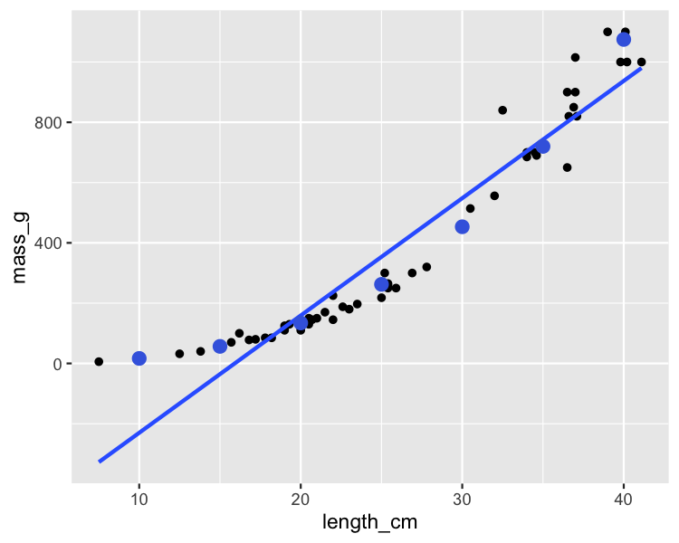
Plot is cramped

ggplot(
  ad_conversion, 
  aes(spent_usd, n_impressions)
) +
  geom_point() +
  geom_smooth(method = "lm", se = FALSE)

A scatter plot of number of impressions versus advertising spend, with a trend line. Most data points are crammed into the bottom left of the plot.

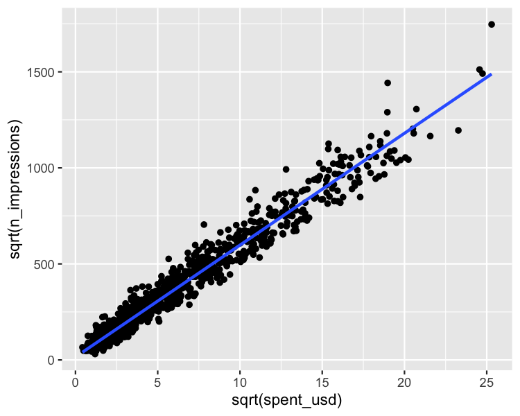
Square root vs square root

ggplot(
  ad_conversion, 
  aes(sqrt(spent_usd), sqrt(n_impressions))
) +
  geom_point() +
  geom_smooth(method = "lm", se = FALSE)

A scatter plot of the square root of the number of impressions versus the square root of the advertising spend, with a trend line. Now the points are more evenly spread throughout the plot.

Modeling and predicting

mdl_ad <- lm(
  sqrt(n_impressions) ~ sqrt(spent_usd), 
  data = ad_conversion
)

explanatory_data <- tibble(
  spent_usd = seq(0, 600, 100)
)

prediction_data <- explanatory_data %>% 
  mutate(
    sqrt_n_impressions = predict(
      mdl_ad, explanatory_data
    ),
    n_impressions = sqrt_n_impressions ^ 2
  )

# A tibble: 7 x 3
  spent_usd sqrt_n_impressions n_impressions
      <dbl>              <dbl>         <dbl>
1         0               15.3          235.
2       100              598.        357289.
3       200              839.        703890.
4       300             1024.       1048771.
5       400             1180.       1392762.
6       500             1318.       1736184.
7       600             1442.       2079202.

Let's practice!

Introduzione alla regressione in R