Perché serve la regressione logistica

Introduzione alla regressione con statsmodels in Python

Maarten Van den Broeck

Content Developer at DataCamp

Dataset churn bancario

has_churned	time_since_first_purchase	time_since_last_purchase
0	0.3993247	-0.5158691
1	-0.4297957	0.6780654
0	3.7383122	0.4082544
0	0.6032289	-0.6990435
...	...	...
risposta	anzianità rapporto	recency attività

¹ https://www.rdocumentation.org/packages/bayesQR/topics/Churn

Churn vs. recency: modello lineare

mdl_churn_vs_recency_lm = ols("has_churned ~ time_since_last_purchase",
                              data=churn).fit()

print(mdl_churn_vs_recency_lm.params)

Intercept                   0.490780
time_since_last_purchase    0.063783
dtype: float64

intercept, slope = mdl_churn_vs_recency_lm.params

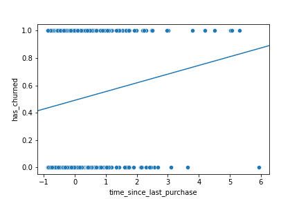
Visualizzare il modello lineare

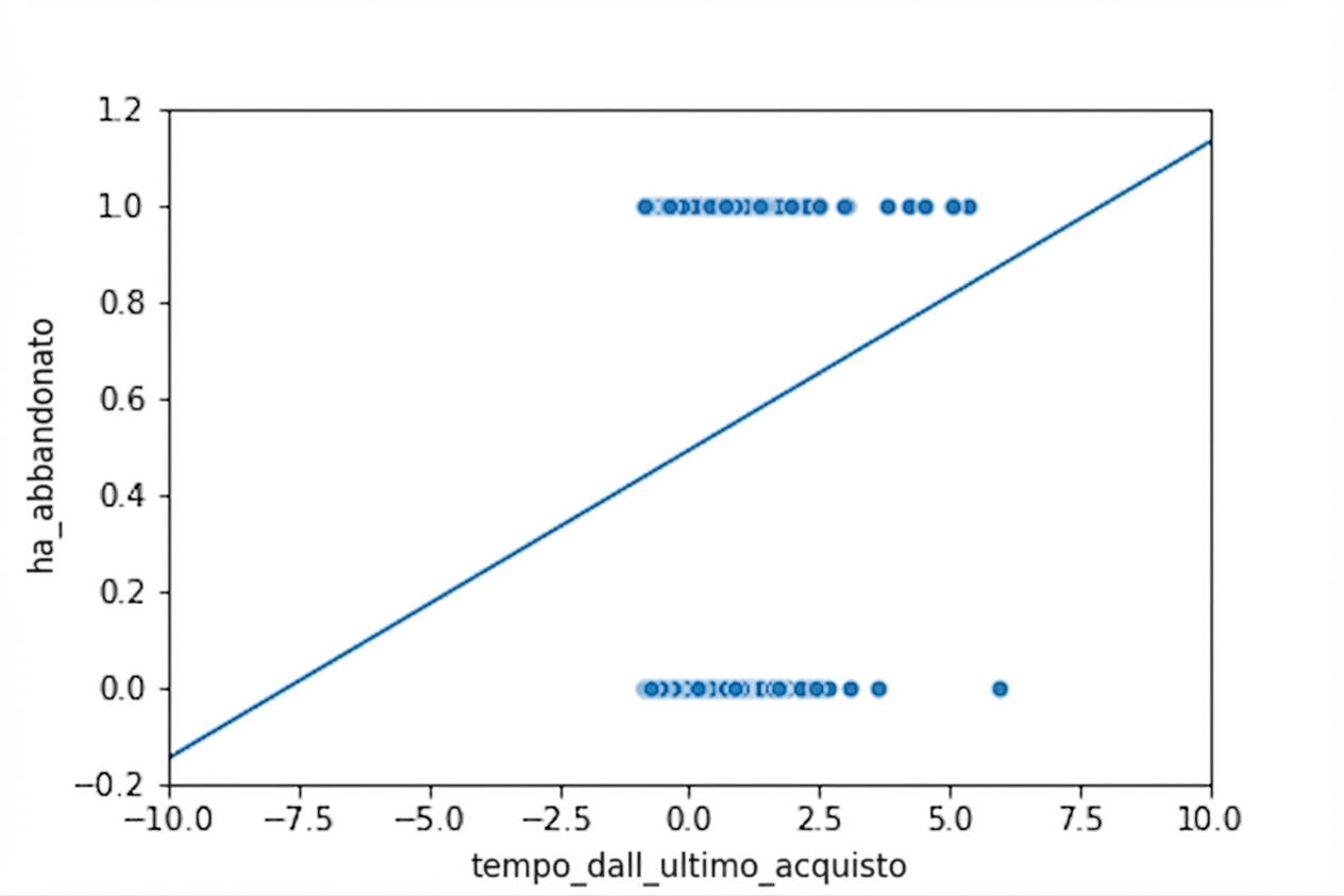
sns.scatterplot(x="time_since_last_purchase",
                y="has_churned",
                data=churn)


plt.axline(xy1=(0, intercept),
           slope=slope)

plt.show()

Uno scatter plot di churn (sì/no) vs tempo dall’ultimo acquisto. Tutti i punti sono su y=0 o y=1. Una retta mostra la probabilità di churn che cresce col tempo dall’ultimo acquisto.

Zoom out

sns.scatterplot(x="time_since_last_purchase",
                y="has_churned",
                data=churn)

plt.axline(xy1=(0,intercept),
           slope=slope)


plt.xlim(-10, 10)
plt.ylim(-0.2, 1.2)

plt.show()

Lo stesso scatter plot. Con assi più ampi, la retta scende sotto 0 e sale sopra 1, cosa impossibile per una probabilità.

Cos’è la regressione logistica?

Un altro tipo di GLM.
Usata quando la variabile risposta è booleana.
Le risposte seguono una curva logistica (a S).

Regressione logistica con logit()

from statsmodels.formula.api import logit
mdl_churn_vs_recency_logit = logit("has_churned ~ time_since_last_purchase",
                                   data=churn).fit()

print(mdl_churn_vs_recency_logit.params)

Intercept                  -0.035019
time_since_last_purchase    0.269215
dtype: float64

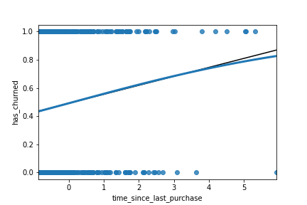
Visualizzare il modello logistico

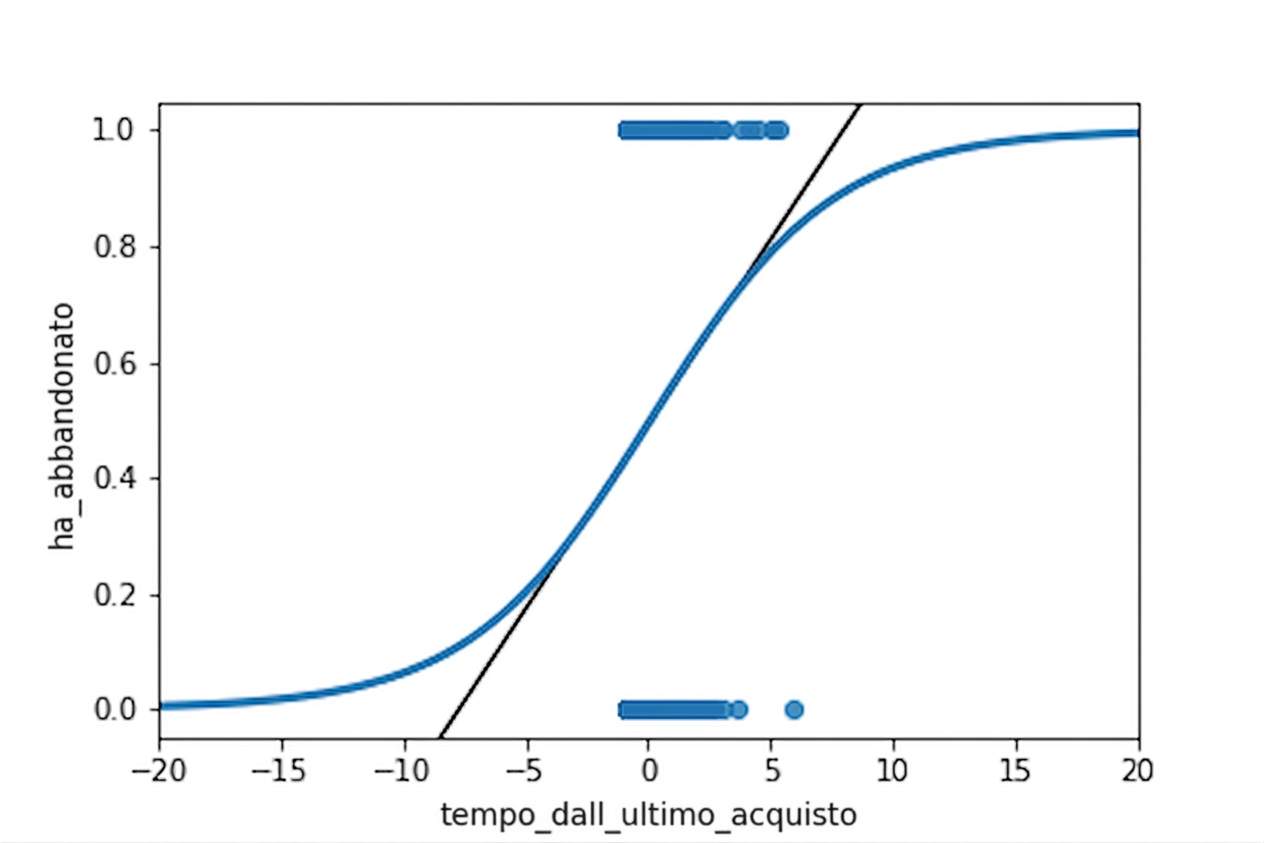
sns.regplot(x="time_since_last_purchase",
            y="has_churned",
            data=churn,
            ci=None,
            logistic=True)

plt.axline(xy1=(0,intercept),
           slope=slope,
           color="black")

plt.show()

Uno scatter plot di churn (sì/no) vs tempo dall’ultimo acquisto. Sono mostrati trend line lineare e logistica; entrambe indicano churn crescente con l’aumento del tempo. Le due curve coincidono quasi sempre, tranne per tempi molto alti.

Zoom out

Lo stesso scatter plot con entrambe le trend line. Assi più ampi mostrano che la curva logistica resta sempre tra 0 e 1.

Ayo berlatih!

Introduzione alla regressione con statsmodels in Python