Lijngrafieken
Introductie tot datavisualisatie met ggplot2

Rick Scavetta
Founder, Scavetta Academy
Beaver
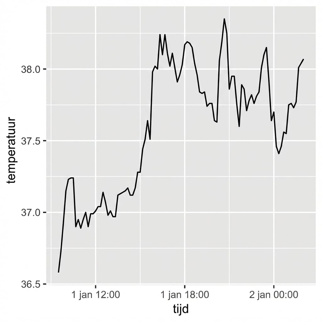
Beaver
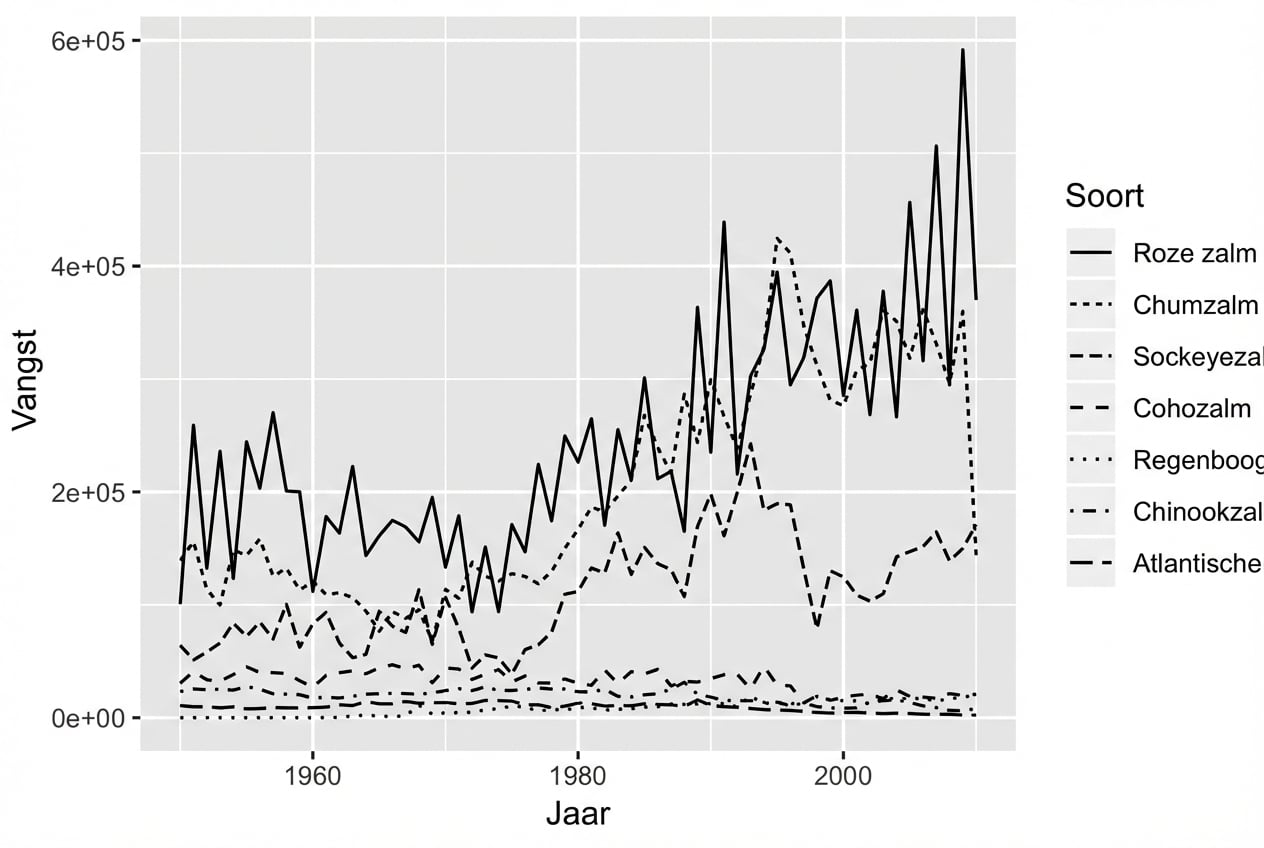
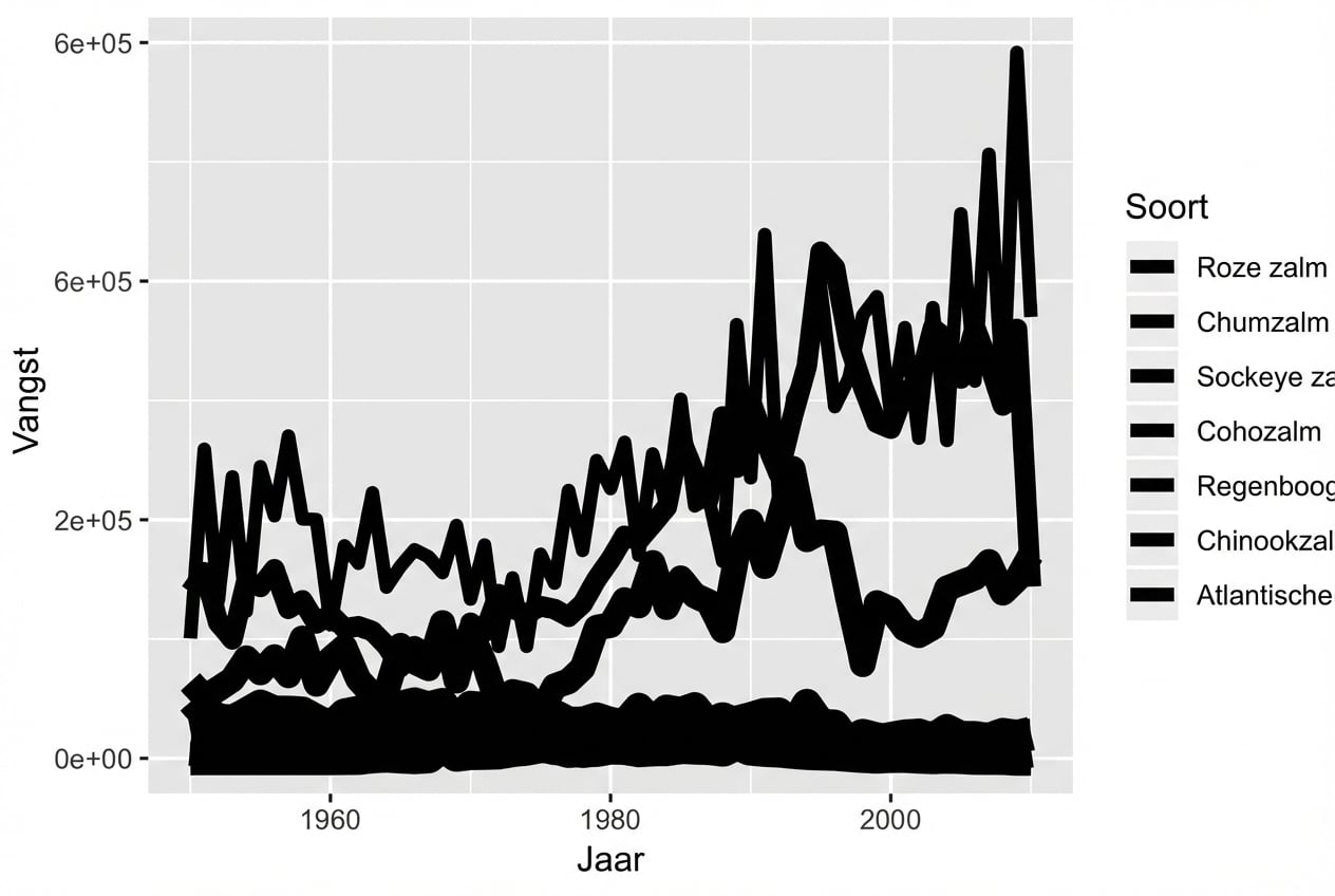
Lijntype-esthetiek
Grootte-esthetiek
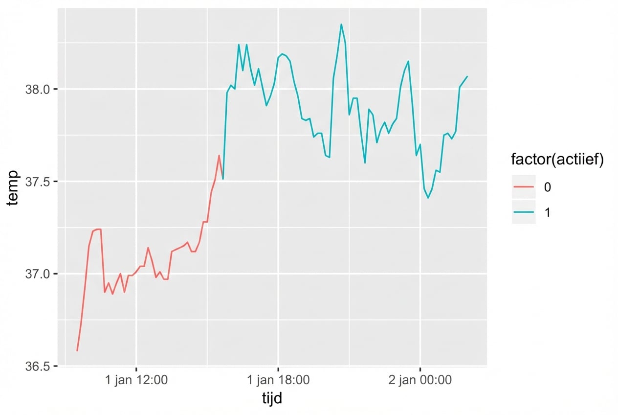
Kleur-esthetiek
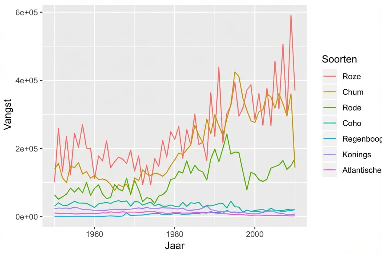
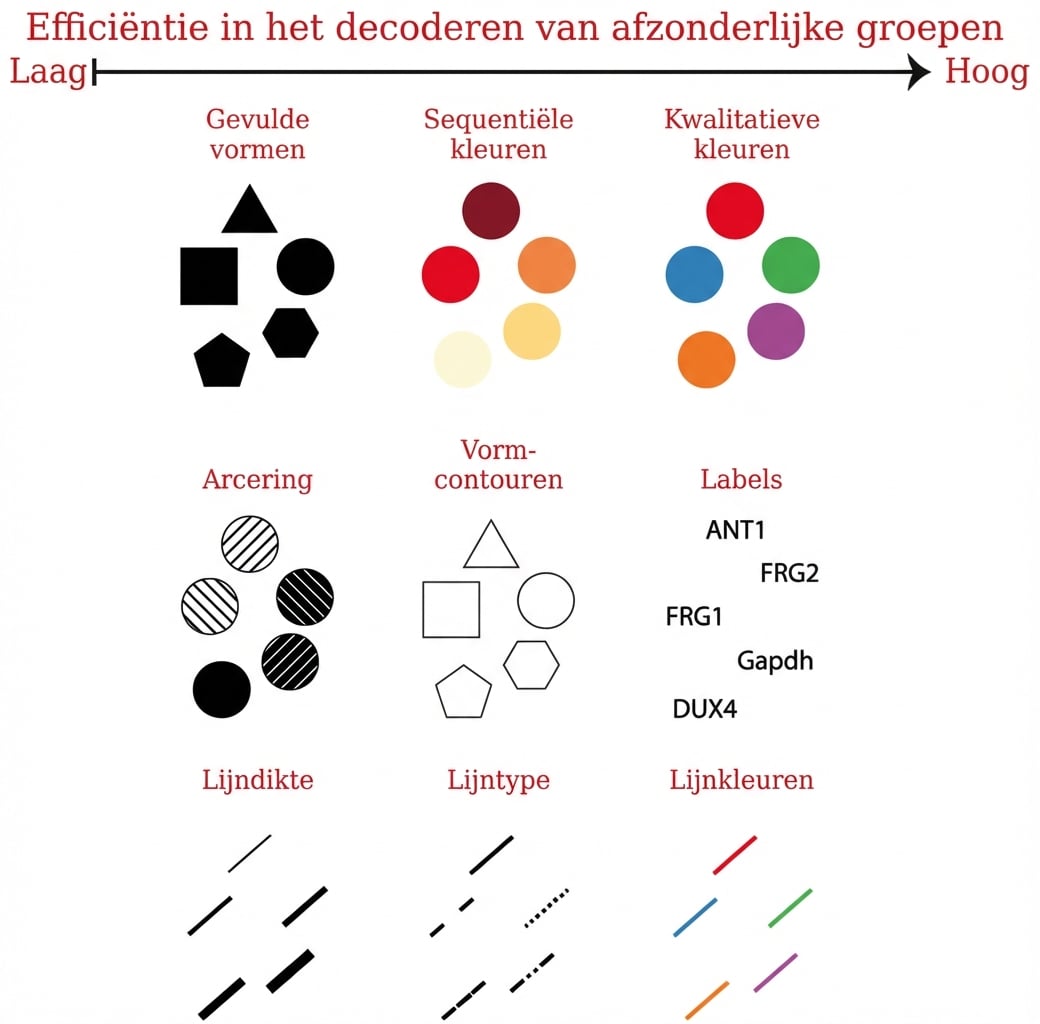
Esthetiek voor categorische variabelen
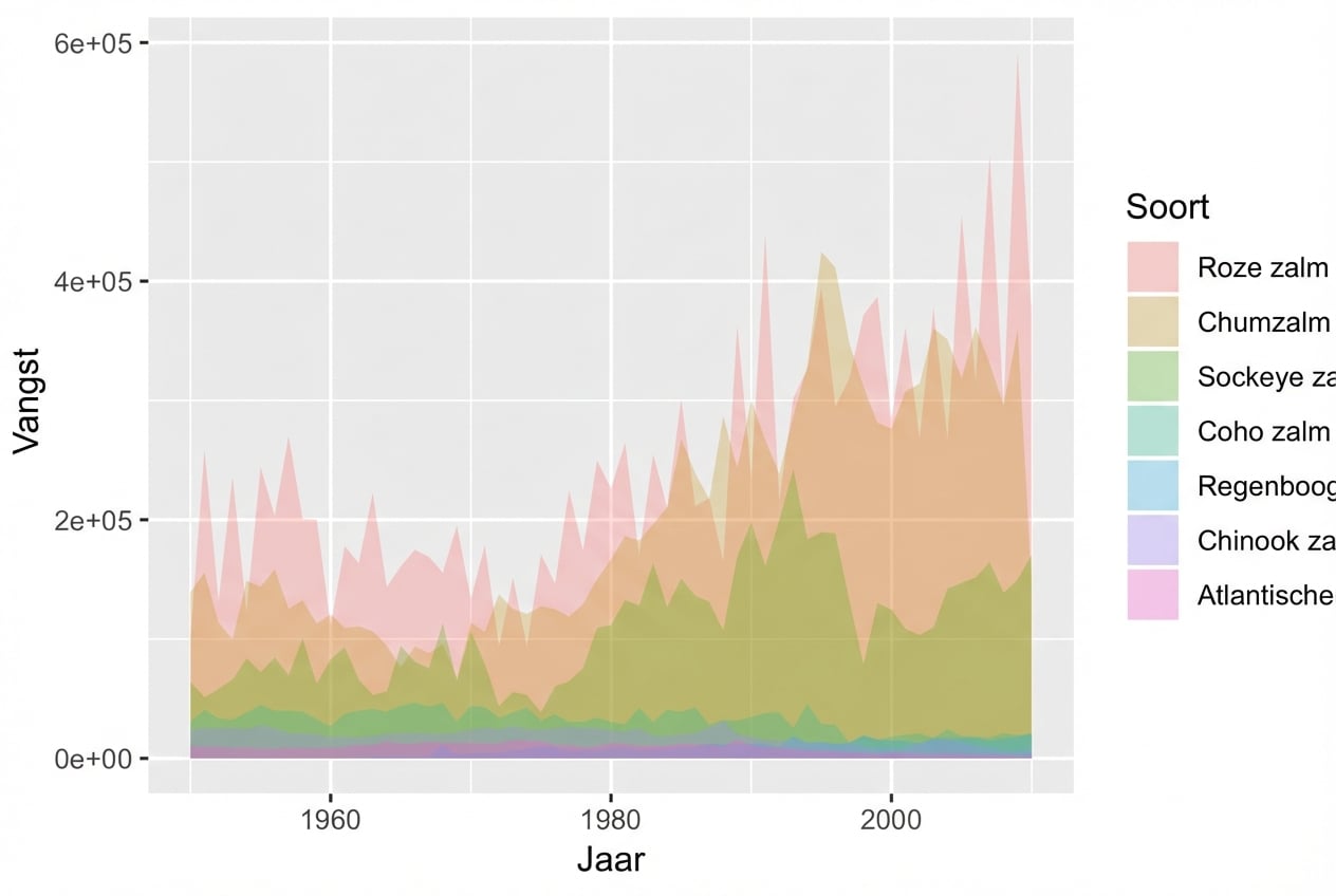
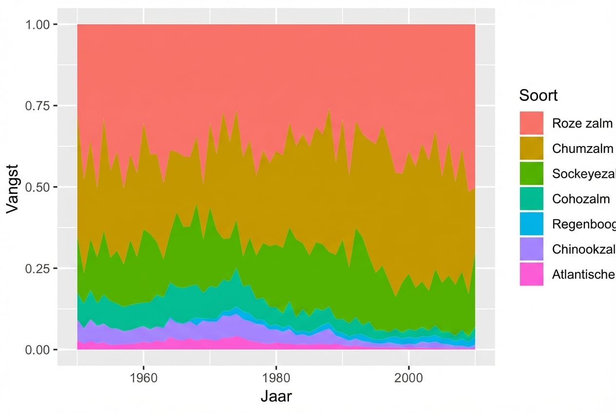
Fill-esthetiek met geom_area()
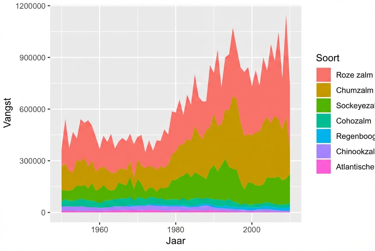
Gebruik van position = "fill"
geom_ribbon()