Spreidingsdiagrammen
Introductie tot datavisualisatie met ggplot2

Rick Scavetta
Founder, Scavetta Academy
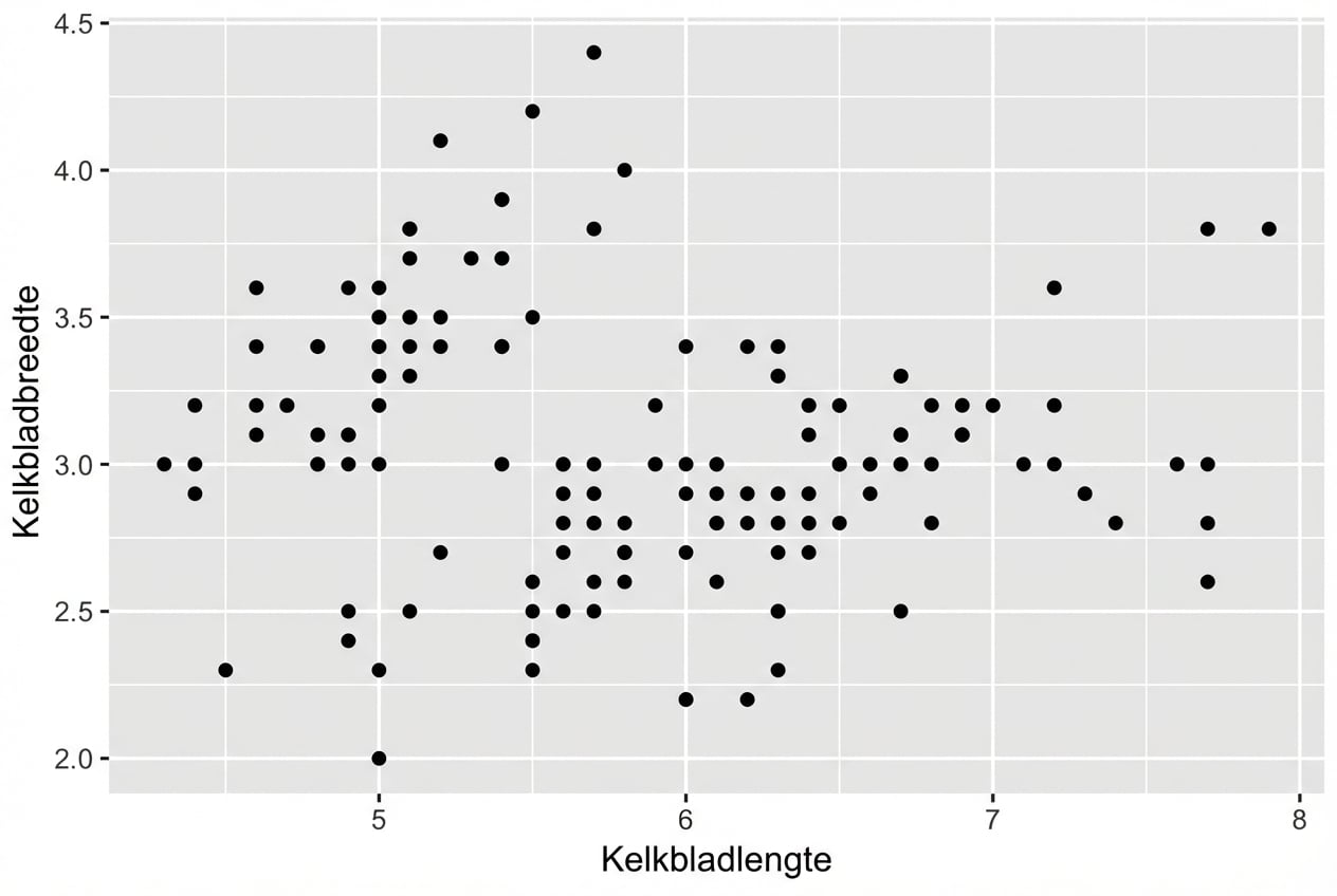
Spreidingsdiagrammen
ggplot(iris, aes(x = Sepal.Length,
                 y = Sepal.Width)) +
  geom_point()
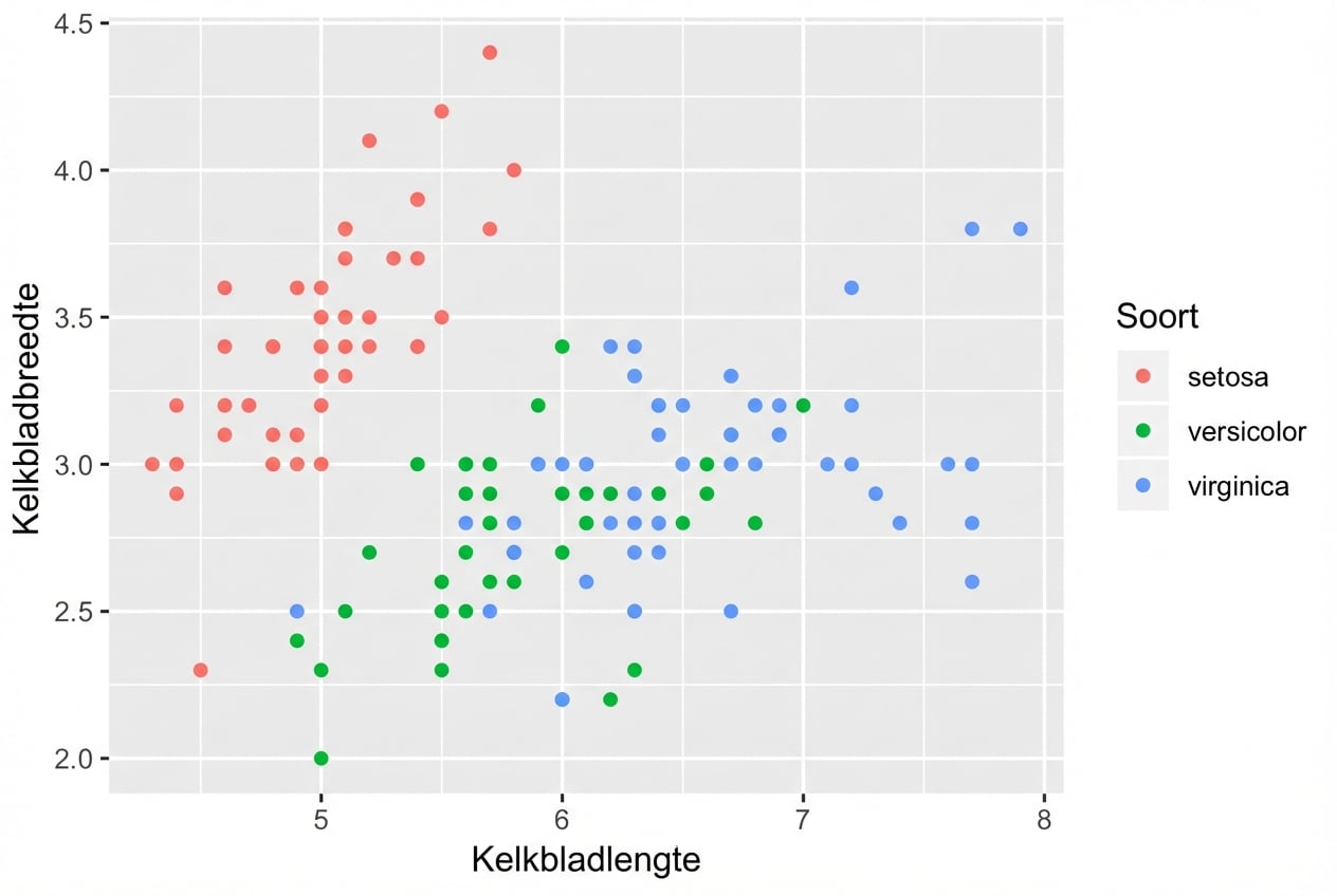
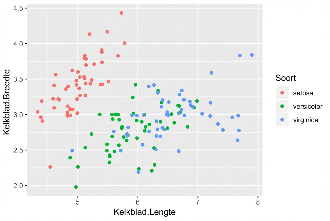
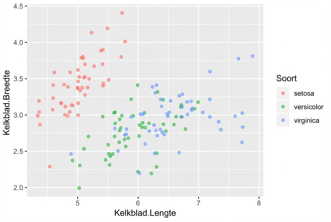
Spreidingsdiagrammen
ggplot(iris, aes(x = Sepal.Length,
                 y = Sepal.Width,
                 col = Species)) +
  geom_point()
Geom-specifieke aesthetic mappings
# Deze geven dezelfde plot!
ggplot(iris, aes(x = Sepal.Length, y = Sepal.Width, col = Species)) +
  geom_point()

ggplot(iris, aes(x = Sepal.Length, y = Sepal.Width)) +
  geom_point(aes(col = Species))
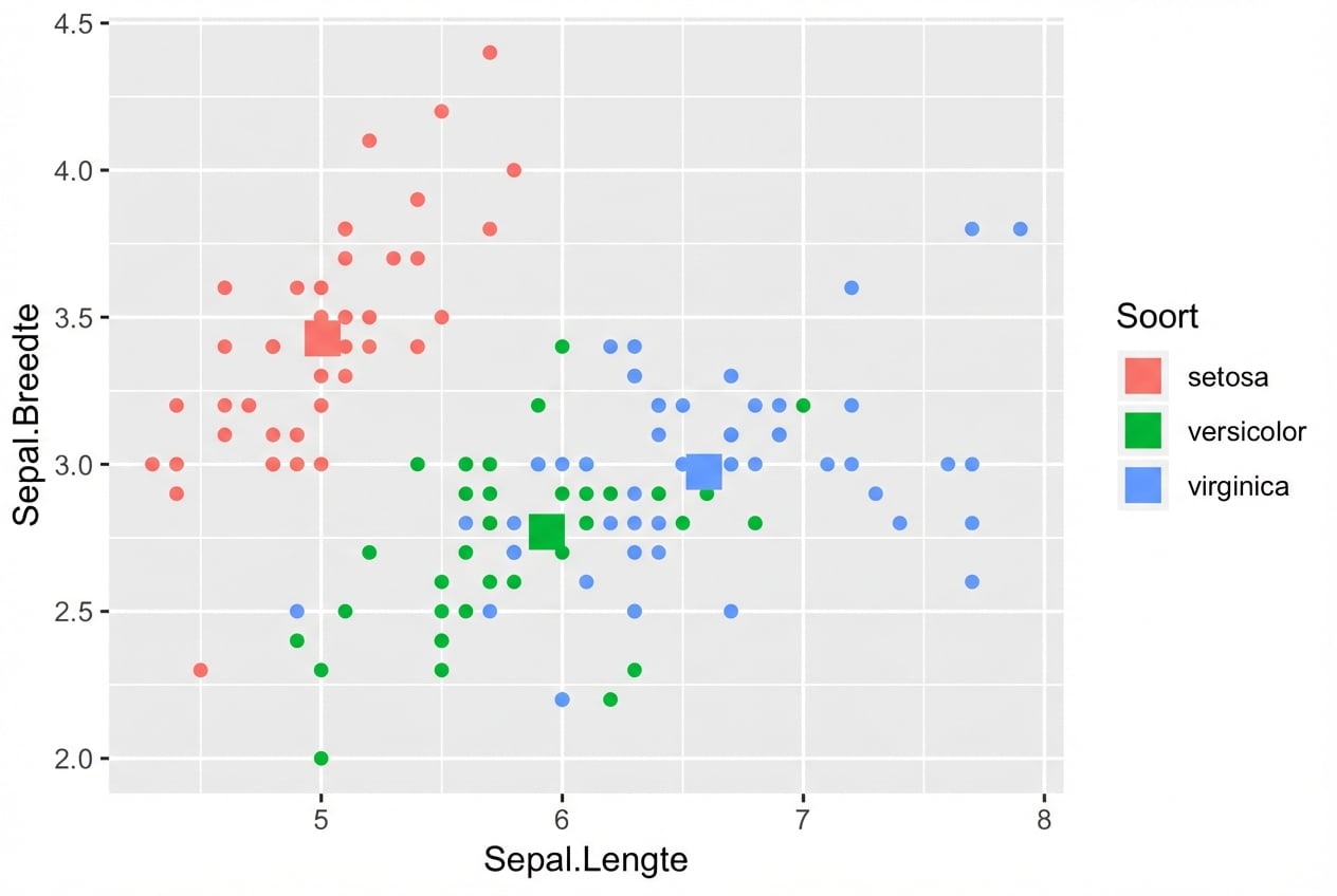
Stuur de aesthetic mappings per layer onafhankelijk aan:
ggplot(iris, aes(x = Sepal.Length, y = Sepal.Width, col = Species)) +
# Neemt data en aes over van ggplot()
geom_point() +
# Andere data, maar geërfde aes
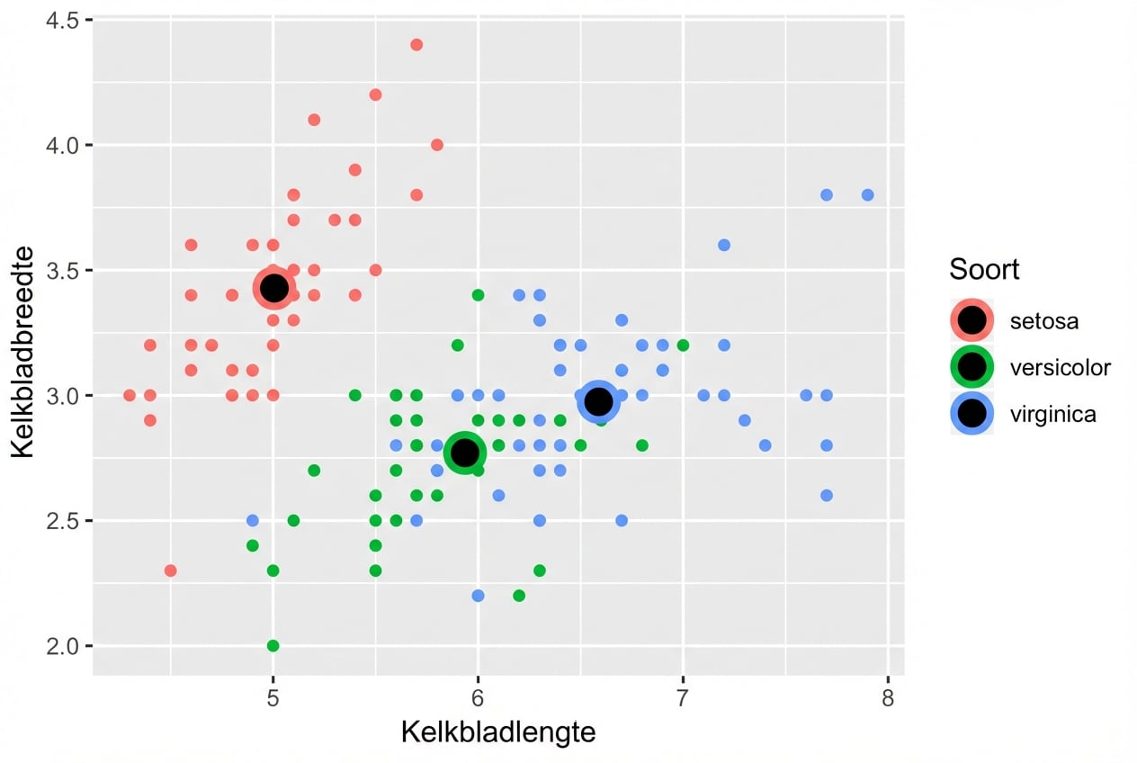
geom_point(data = iris.summary, shape = 15, size = 5)
Waardes voor attribuut shape
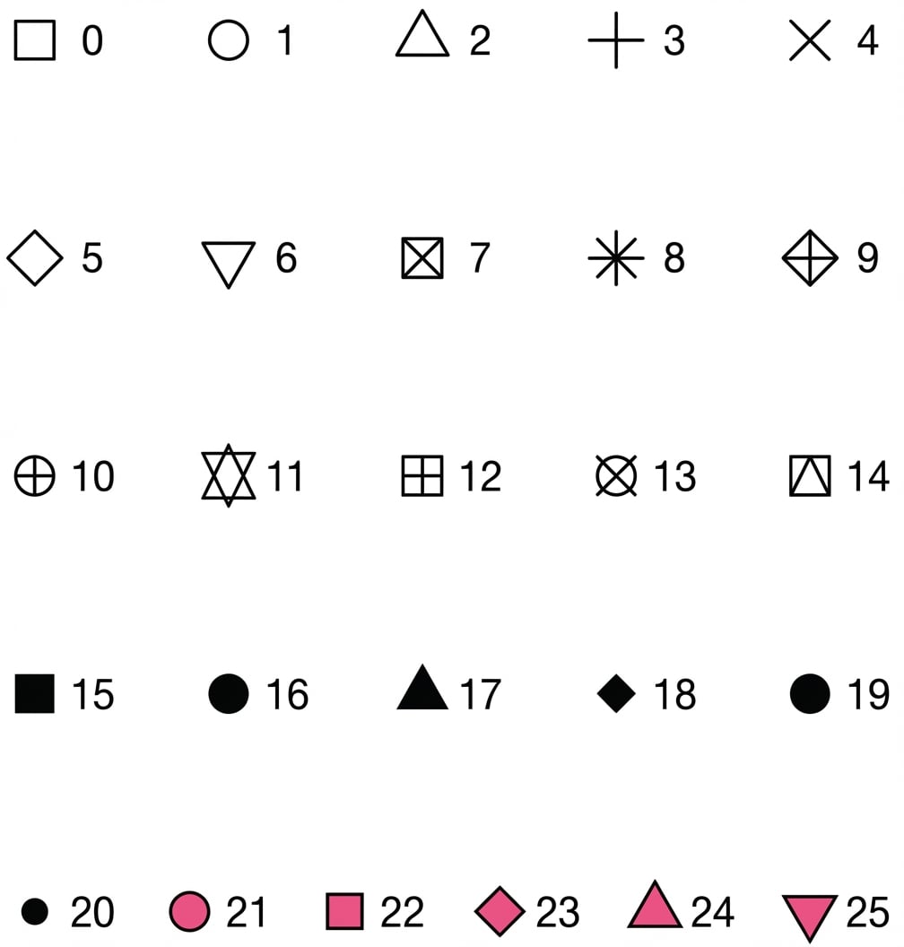
Voorbeeld
ggplot(iris, aes(x = Sepal.Length, y = Sepal.Width, col = Species)) +
  geom_point() +
  geom_point(data = iris.summary, shape = 21, size = 5,
             fill = "black", stroke = 2)
Ad-hoc statistiek door ggplot2
- Zie cursus 2 voor de stats-laag.
- Let op: plot niet alleen het gemiddelde zonder spreidingsmaat, bv. de standaarddeviatie.
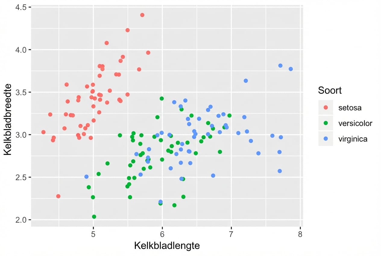
position = "jitter"
ggplot(iris, aes(x = Sepal.Length, y = Sepal.Width, col = Species)) +
  geom_point(position = "jitter")
geom_jitter()
Een snelkoppeling voor geom_point(position = "jitter")
ggplot(iris, aes(x = Sepal.Length, y = Sepal.Width, col = Species)) +
  geom_jitter()
Vergeet alpha niet aan te passen
- Combineer jitter met alpha-blending indien nodig
ggplot(iris, aes(x = Sepal.Length, y = Sepal.Width, col = Species)) +
  geom_jitter(alpha = 0.6)
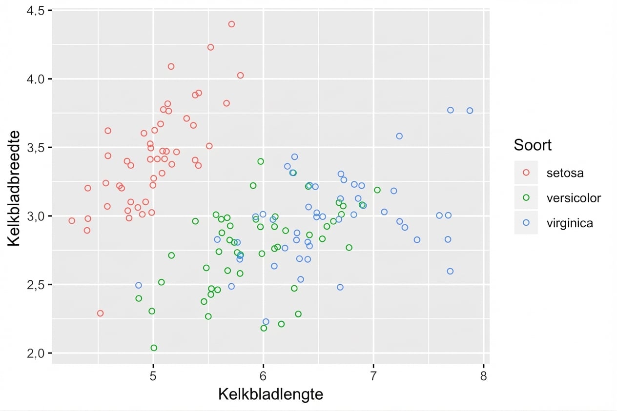
Holle cirkels helpen ook
shape = 1is een holle cirkel.- Alpha-blending is dan vaak niet nodig.
ggplot(iris, aes(x = Sepal.Length, y = Sepal.Width, col = Species)) +
  geom_jitter(shape = 1)