Waarom je logistische regressie nodig hebt

Introductie tot regressie in R

Richie Cotton

Data Evangelist at DataCamp

Bank-churn-dataset

has_churned	time_since_first_purchase	time_since_last_purchase
0	0.3993247	-0.5158691
1	-0.4297957	0.6780654
0	3.7383122	0.4082544
0	0.6032289	-0.6990435
...	...	...
response	duur van relatie	recency van activiteit

¹ https://www.rdocumentation.org/packages/bayesQR/topics/Churn

Churn vs. recency: een lineair model

mdl_churn_vs_recency_lm <- lm(has_churned ~ time_since_last_purchase, data = churn)

Call:
lm(formula = has_churned ~ time_since_last_purchase, data = churn)

Coefficients:
             (Intercept)  time_since_last_purchase  
                 0.49078                   0.06378

coeffs <- coefficients(mdl_churn_vs_recency_lm)
intercept <- coeffs[1]
slope <- coeffs[2]

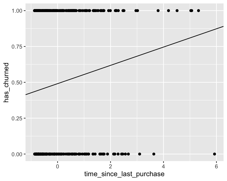
Het lineaire model visualiseren

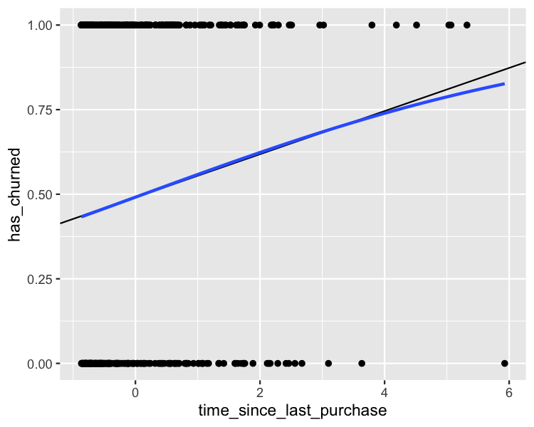
ggplot(
  churn, 
  aes(time_since_last_purchase, has_churned)
) +
  geom_point() +
  geom_abline(intercept = intercept, slope = slope)

Voorspellingen zijn kansen op churn, geen hoeveelheden churn.

Een spreidingsdiagram van wel/niet klantvertrek versus tijd sinds laatste aankoop. Alle punten liggen op y = 0 of y = 1. Een lineaire trendlijn toont een stijgende churn-kans bij meer tijd sinds laatste aankoop.

Uitzoomen

ggplot(
  churn, 
  aes(days_since_last_purchase, has_churned)
) +
  geom_point() +
  geom_abline(intercept = intercept, slope = slope) +
  xlim(-10, 10) +
  ylim(-0.2, 1.2)

Hetzelfde spreidingsdiagram, uitgezoomd. De lineaire trendlijn gaat onder y = 0 en boven y = 1, wat onmogelijk zou moeten zijn.

Wat is logistische regressie?

Een ander type gegeneraliseerd lineair model.
Gebruik je als de responsvariabele logisch is.
Respons volgt een logistische (S-vormige) curve.

Lineaire regressie met glm()

glm(has_churned ~ time_since_last_purchase, data = churn, family = gaussian)

Call:  glm(formula = has_churned ~ time_since_last_purchase, family = gaussian, 
    data = churn)

Coefficients:
             (Intercept)  time_since_last_purchase  
                 0.49078                   0.06378  

Degrees of Freedom: 399 Total (i.e. Null);  398 Residual
Null Deviance:        100 
Residual Deviance: 98.02     AIC: 578.7

Logistische regressie: glm() met binomiale family

mdl_recency_glm <- glm(has_churned ~ time_since_last_purchase, data = churn, family = binomial)

Call:  glm(formula = has_churned ~ time_since_last_purchase, family = binomial, 
    data = churn)

Coefficients:
             (Intercept)  time_since_last_purchase  
                -0.03502                   0.26921  

Degrees of Freedom: 399 Total (i.e. Null);  398 Residual
Null Deviance:        554.5 
Residual Deviance: 546.4     AIC: 550.4

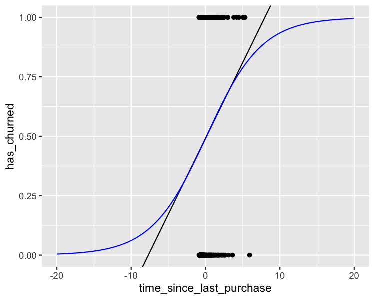
De logistieke modelcurve visualiseren

ggplot(
  churn, 
  aes(time_since_last_purchase, has_churned)
) +
  geom_point() +
  geom_abline(
    intercept = intercept, slope = slope
  ) +
  geom_smooth(
    method = "glm", 
    se = FALSE, 
    method.args = list(family = binomial)
  )

Een spreidingsdiagram van wel/niet klantvertrek versus tijd sinds laatste aankoop. Lineaire en logistische trendlijnen tonen beide stijgende vertrek-kans bij meer tijd sinds laatste aankoop. Ze liggen dicht bij elkaar, behalve bij hoge waarden van tijd sinds laatste aankoop.

Uitzoomen

Het spreidingsdiagram van wel/niet klantvertrek versus tijd sinds laatste aankoop, met beide trendlijnen. De assen zijn verder uitgezoomd en tonen dat de logistische lijn altijd binnen het bereik 0–1 blijft.

Laten we oefenen!

Introductie tot regressie in R