Statistieken buiten geoms
Gevorderde datavisualisatie met ggplot2

Rick Scavetta
Founder, Scavetta Academy
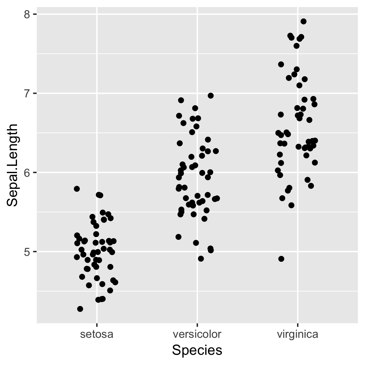
Basisplot
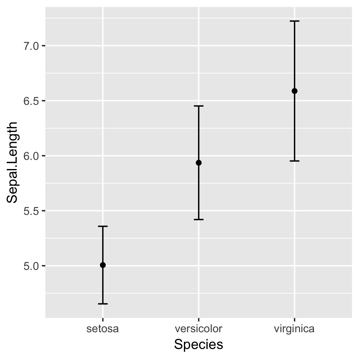
stat_summary()
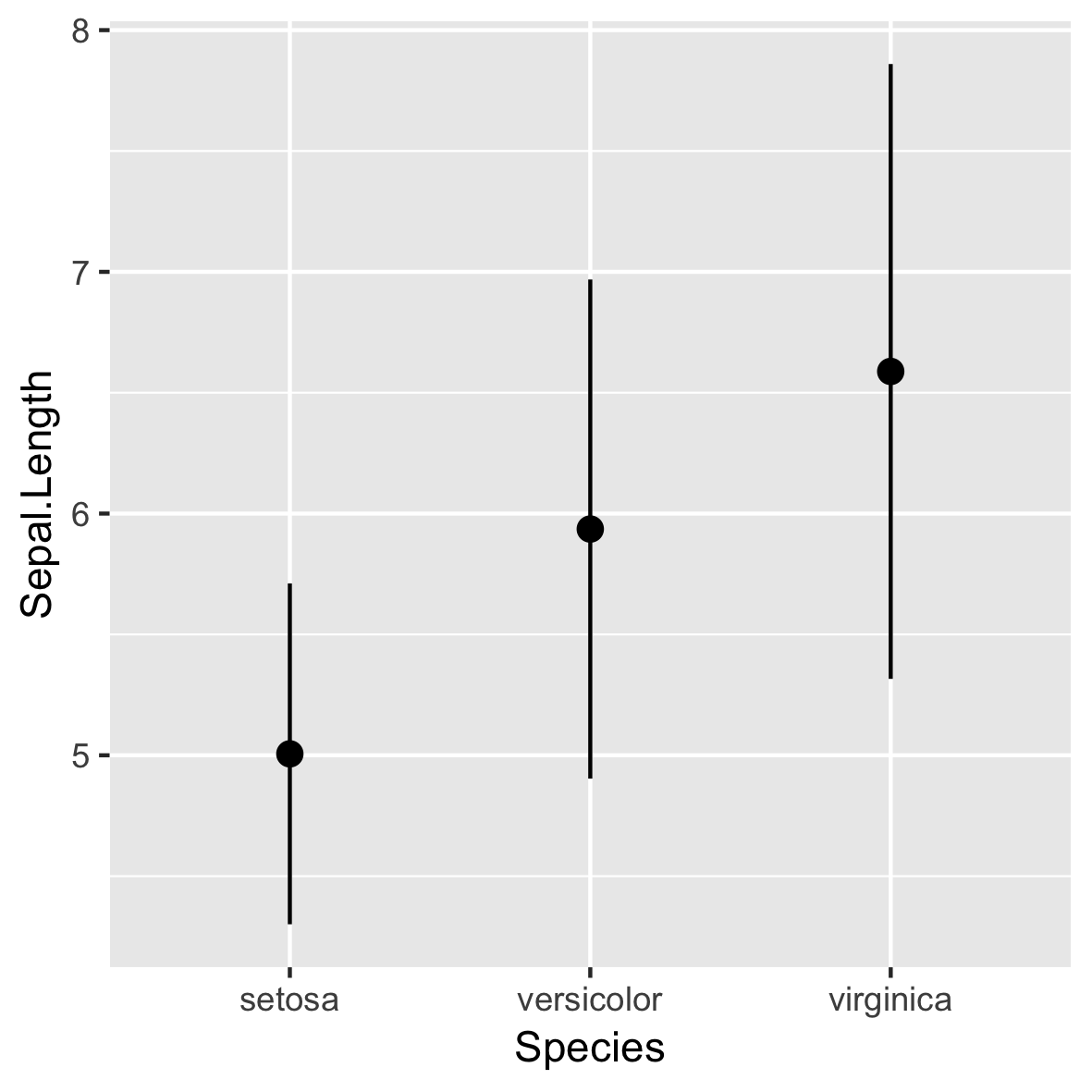
stat_summary()
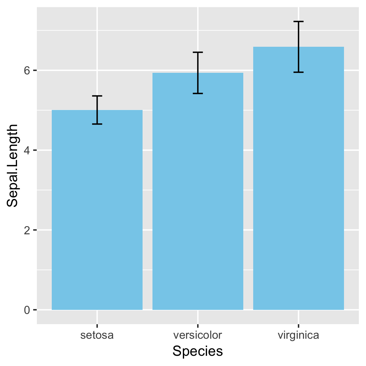
Niet aanbevolen!
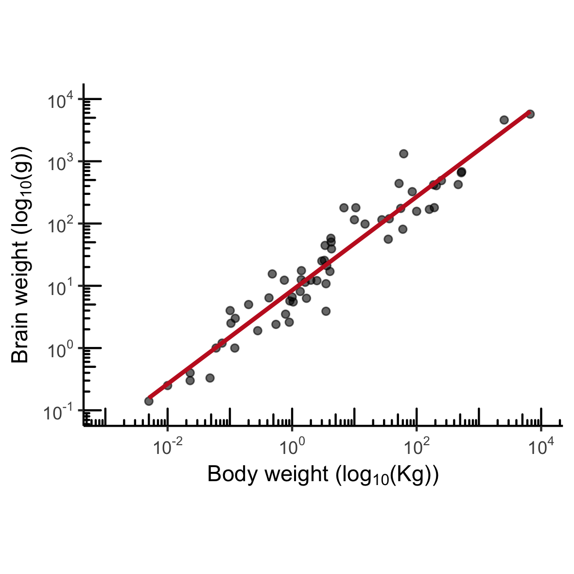
MASS::mammals
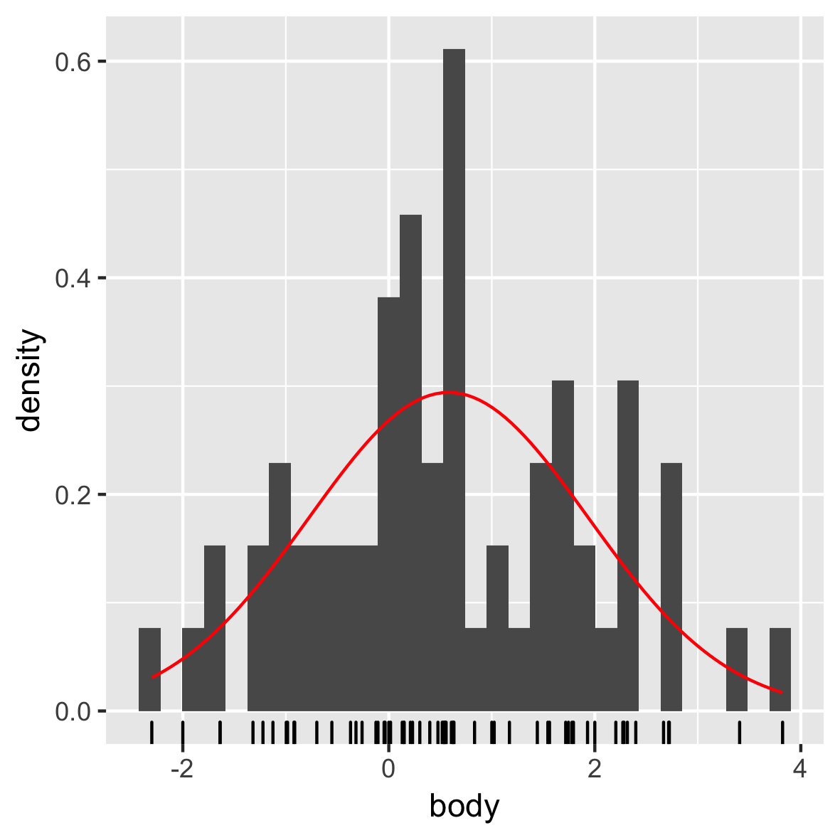
Normale verdeling
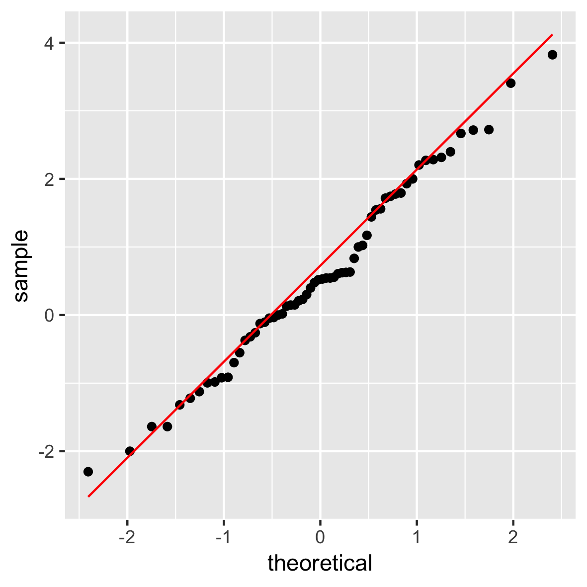
QQ-plot
Gevorderde datavisualisatie met ggplot2
Rick Scavetta
Founder, Scavetta Academy
Niet aanbevolen!

