Modelprestatie visualiseren
Modelleren met tidymodels in R

David Svancer
Data Scientist
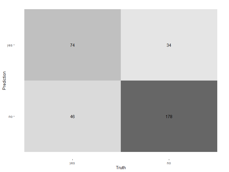
De confusion matrix plotten
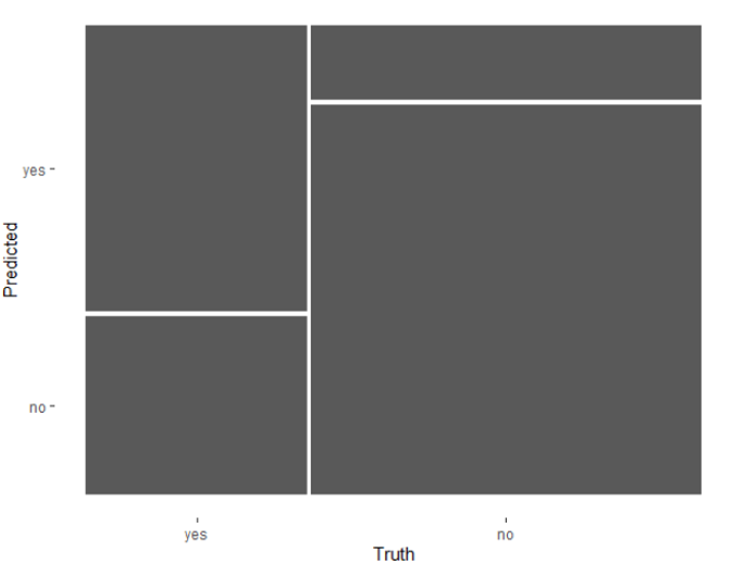
Mozaïekdiagram
Mozaïekdiagram
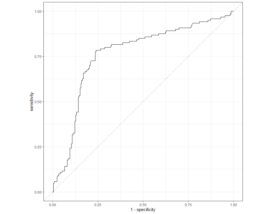
Prestatie over drempels visualiseren
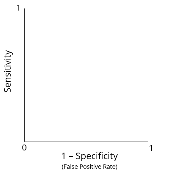
Prestatie over drempels visualiseren
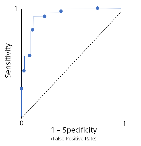
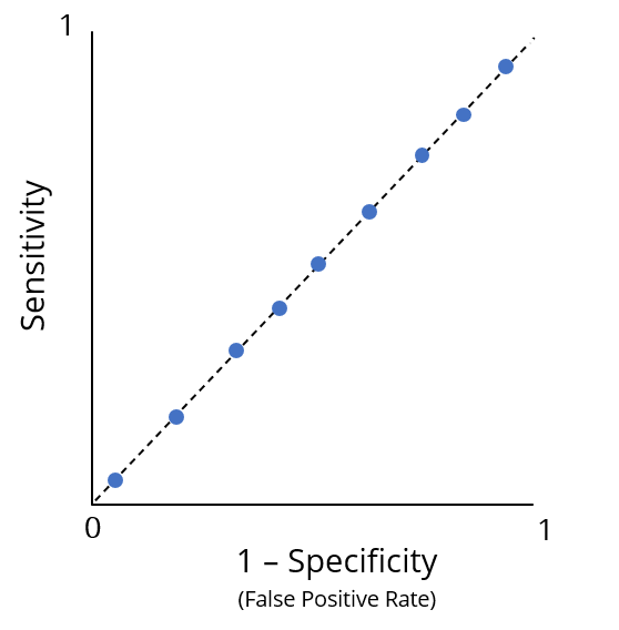
ROC-curves
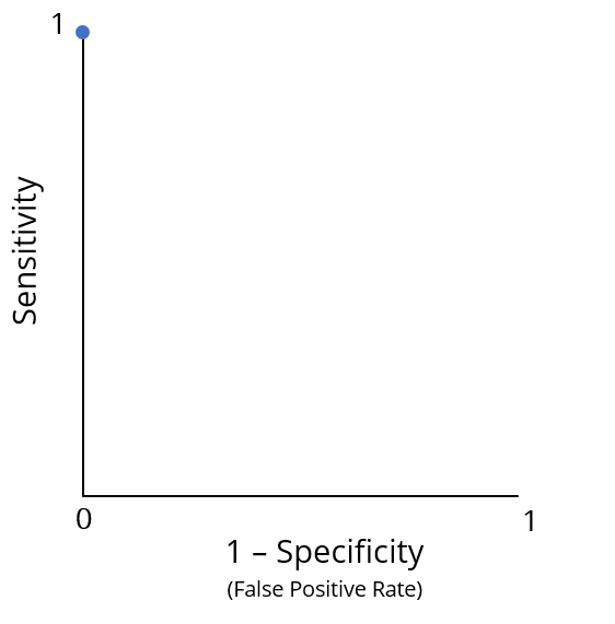
ROC-curves
De ROC-curve samenvatten
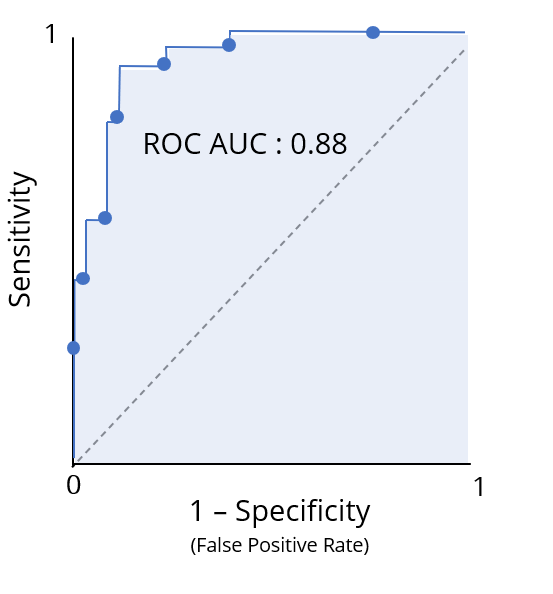
De ROC-curve plotten