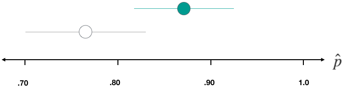
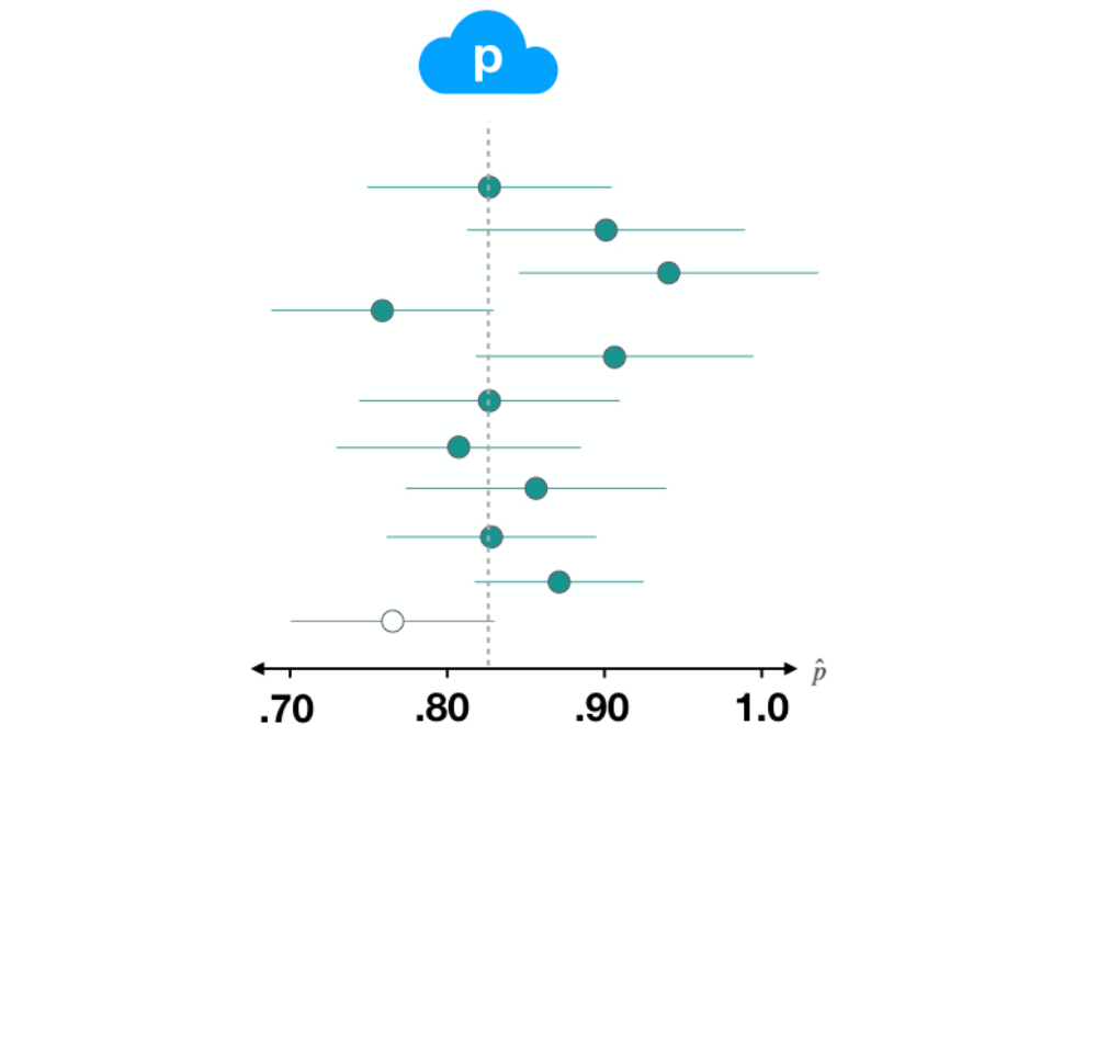
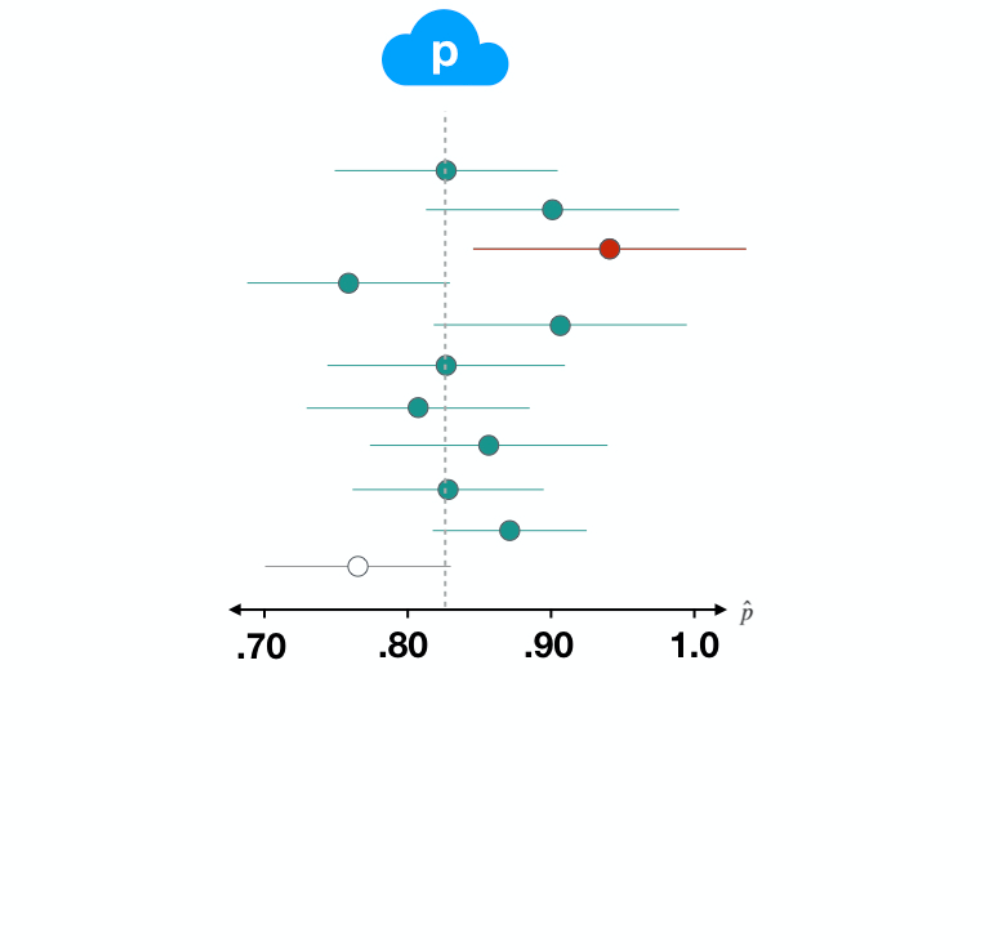
Een betrouwbaarheidsinterval interpreteren
Inferentie voor categorische gegevens in R

Andrew Bray
Assistant Professor of Statistics at Reed College
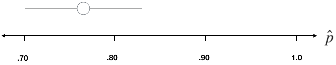
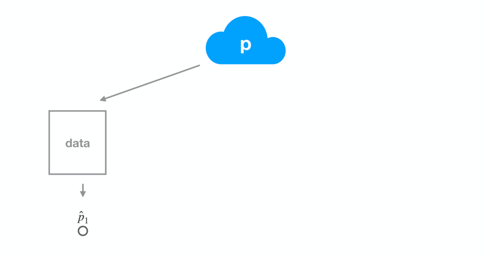
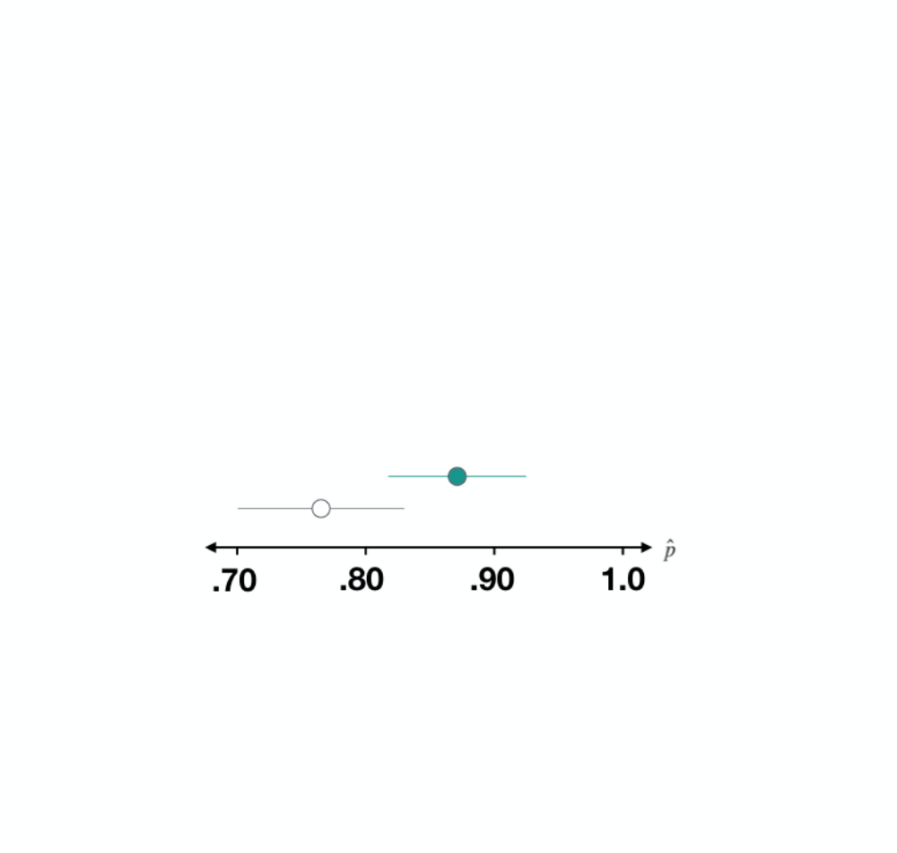
Dataset 1


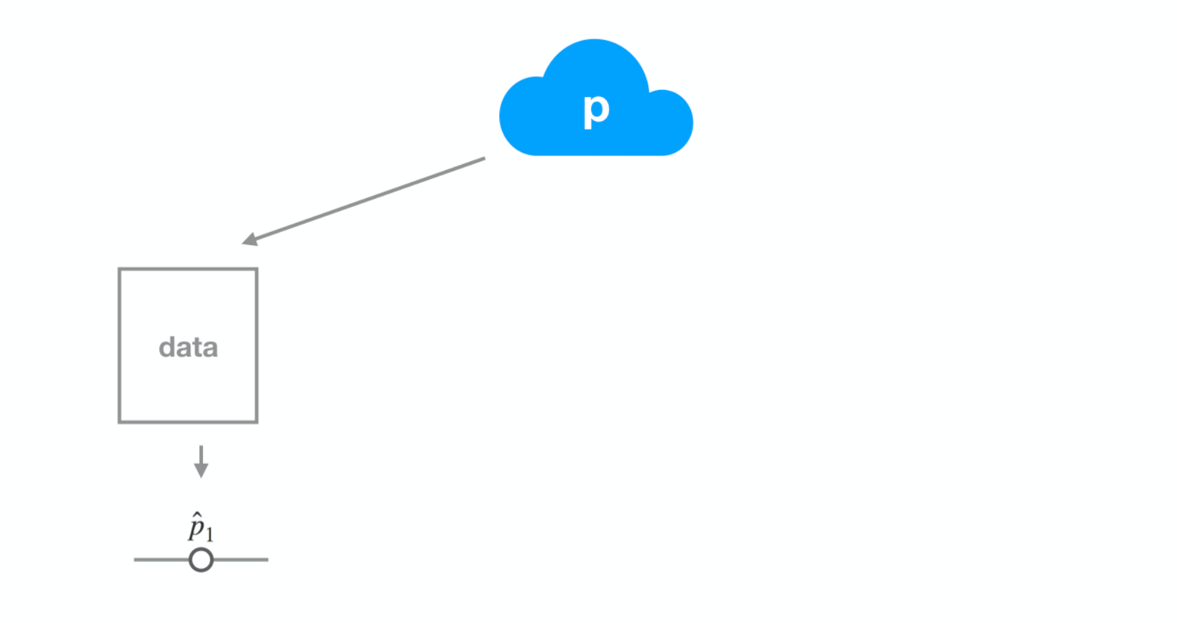


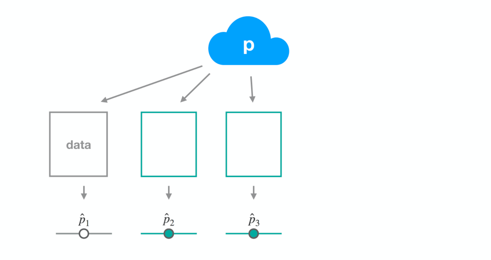
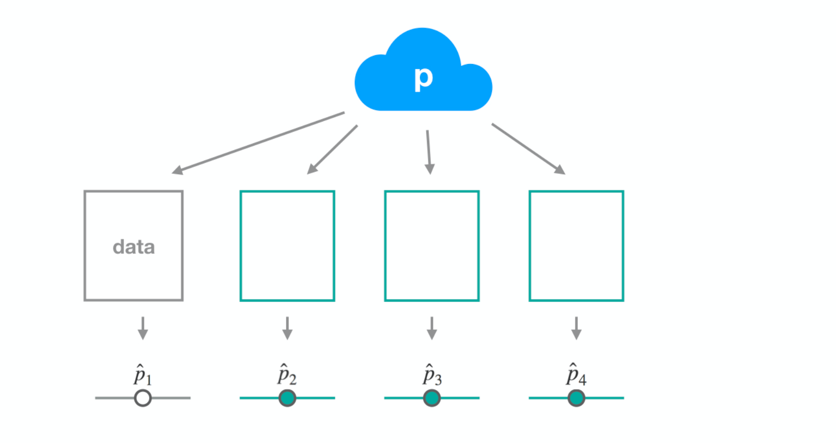
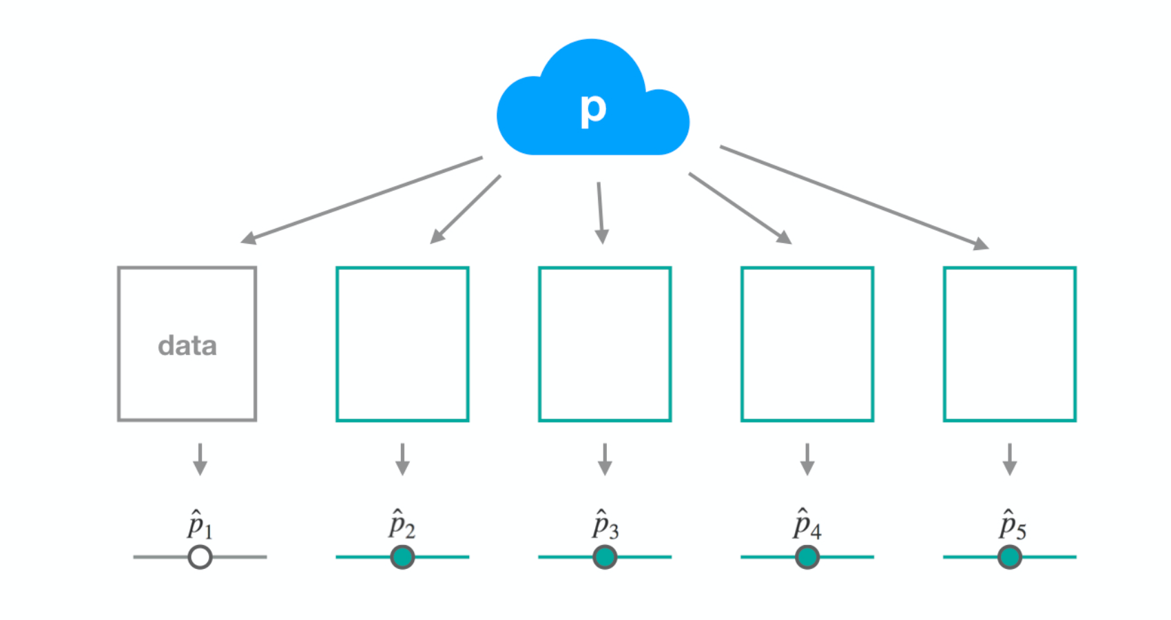
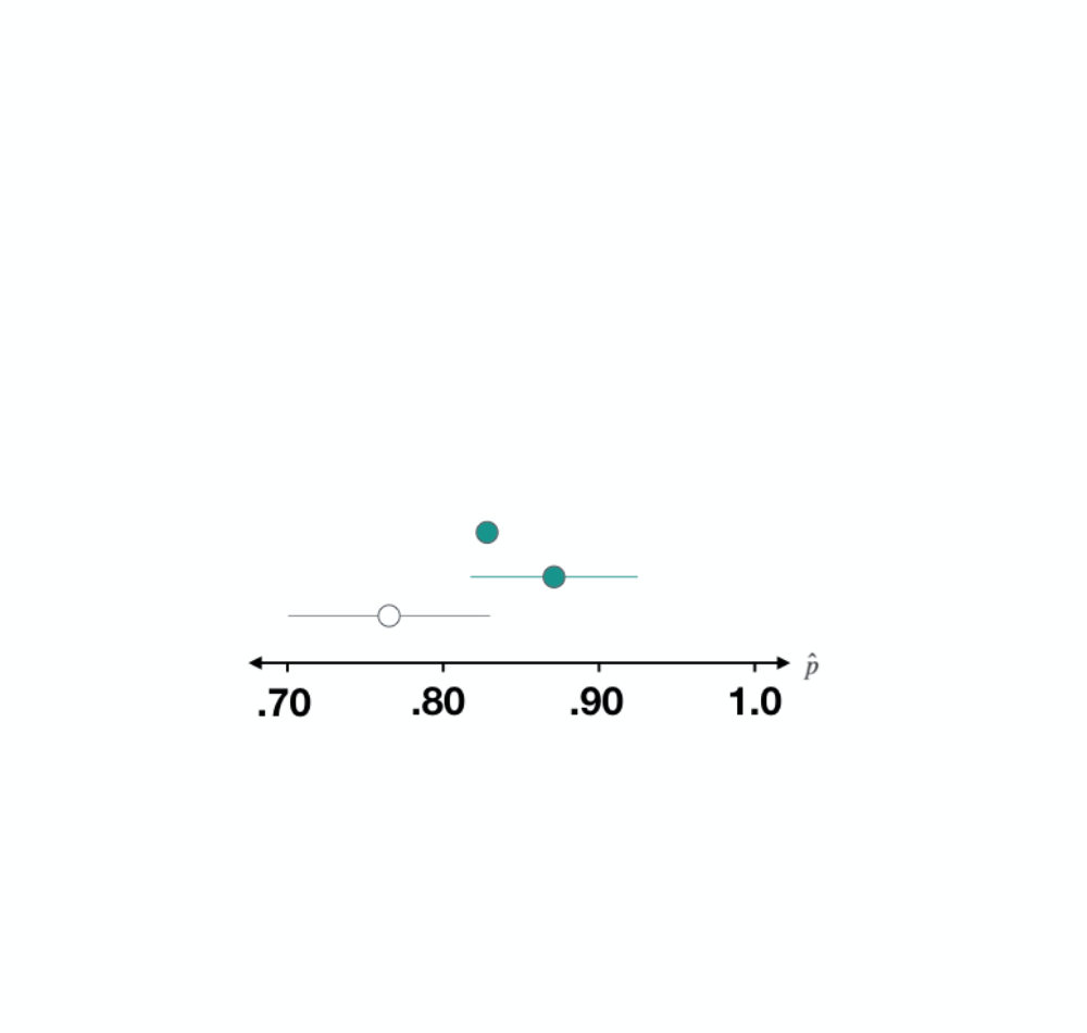
Dataset 2
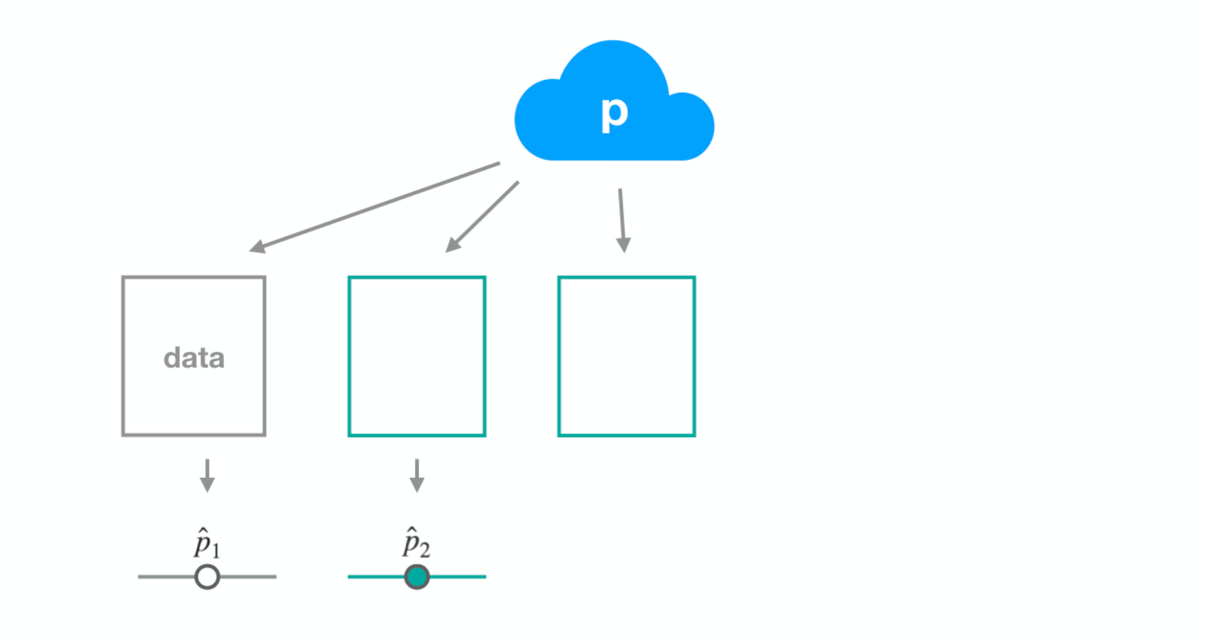
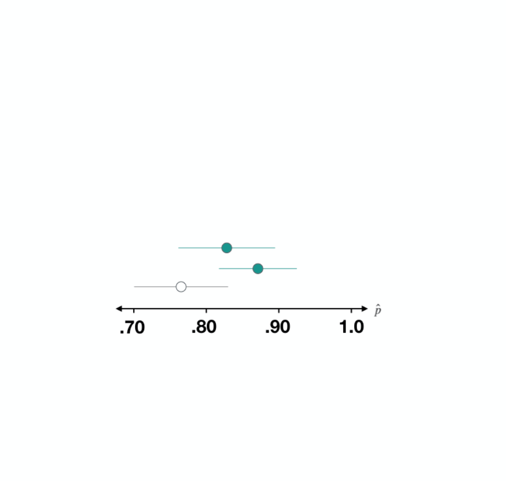
Dataset 3
Dataset 3
Dataset 3
Dataset 3
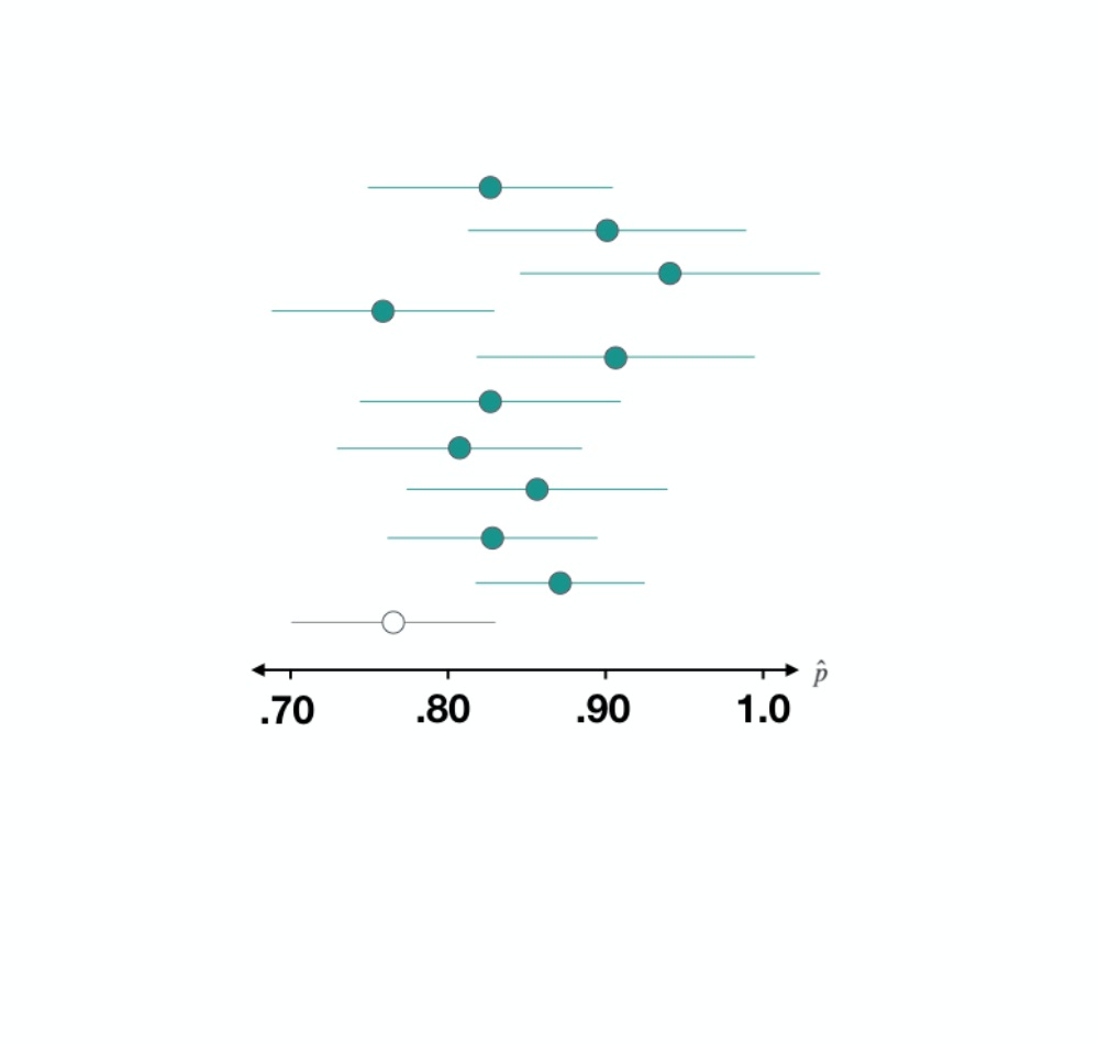
Dataset 3
Dataset 3
Inferentie voor categorische gegevens in R
Andrew Bray
Assistant Professor of Statistics at Reed College

