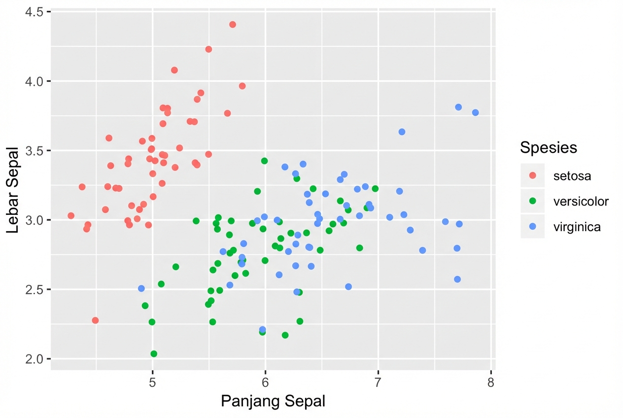
Scatter plot
Pengantar Visualisasi Data dengan ggplot2

Rick Scavetta
Founder, Scavetta Academy
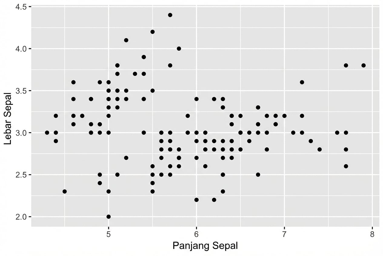
Scatter plot
ggplot(iris, aes(x = Sepal.Length,
                 y = Sepal.Width)) +
  geom_point()
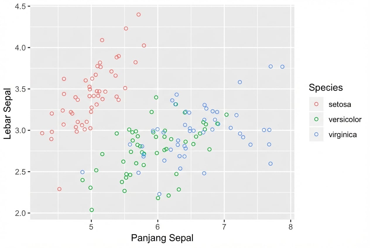
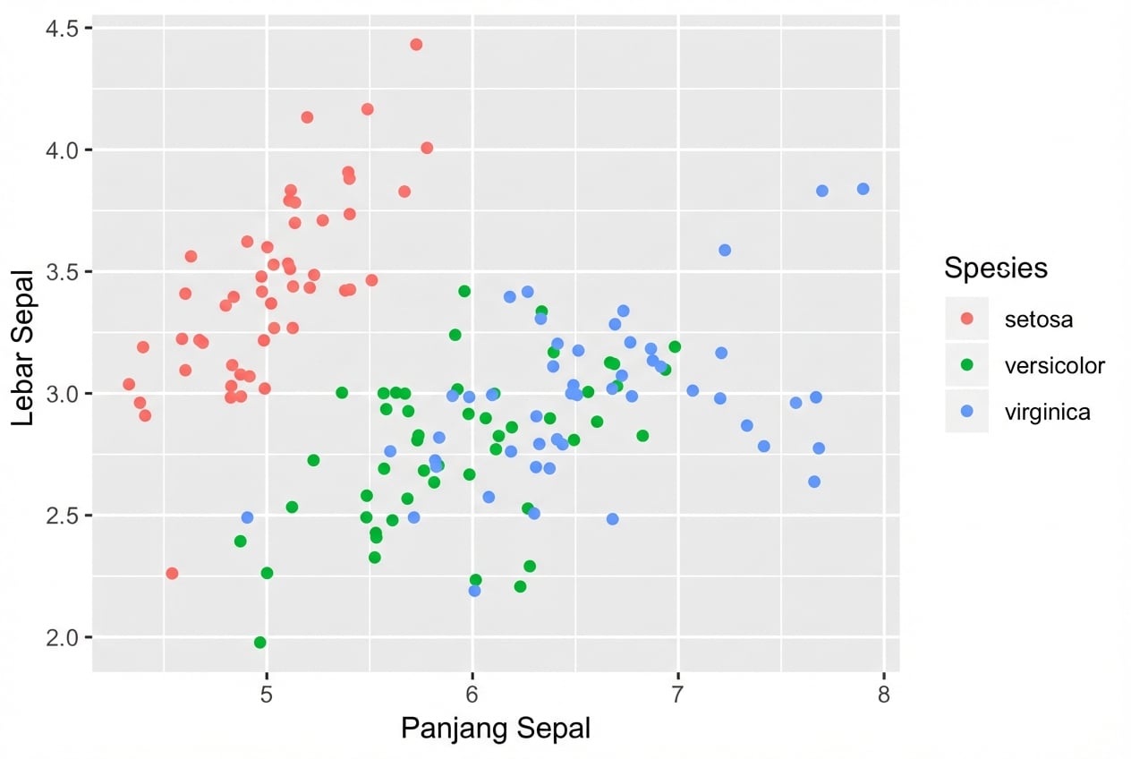
Scatter plot
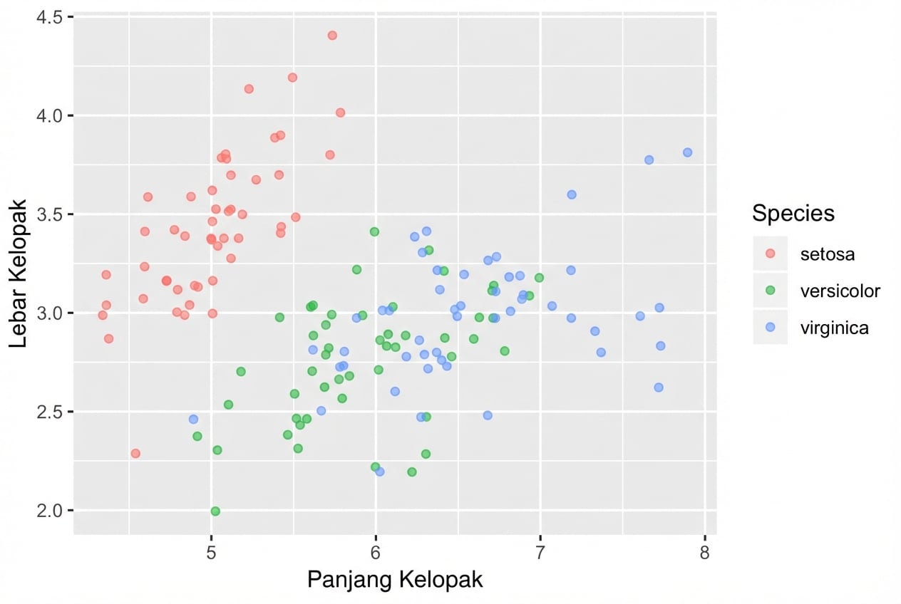
ggplot(iris, aes(x = Sepal.Length,
                 y = Sepal.Width,
                 col = Species)) +
  geom_point()
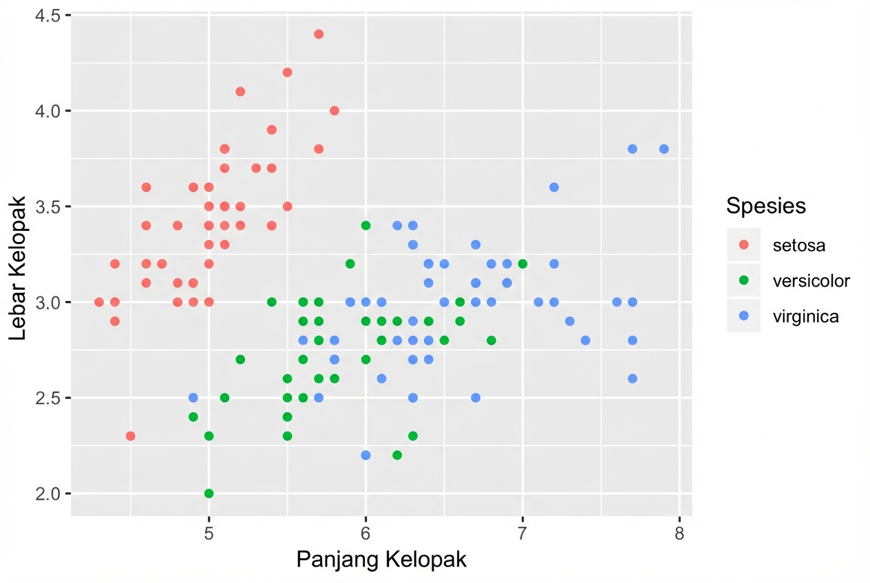
Pemetaan estetika khusus geom
# Hasilnya plot yang sama!
ggplot(iris, aes(x = Sepal.Length, y = Sepal.Width, col = Species)) +
  geom_point()

ggplot(iris, aes(x = Sepal.Length, y = Sepal.Width)) +
  geom_point(aes(col = Species))
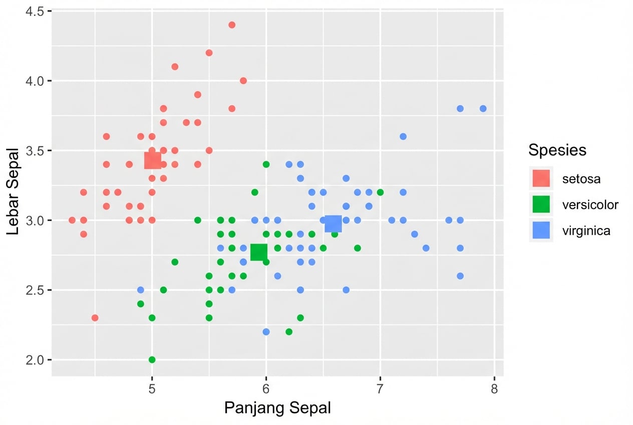
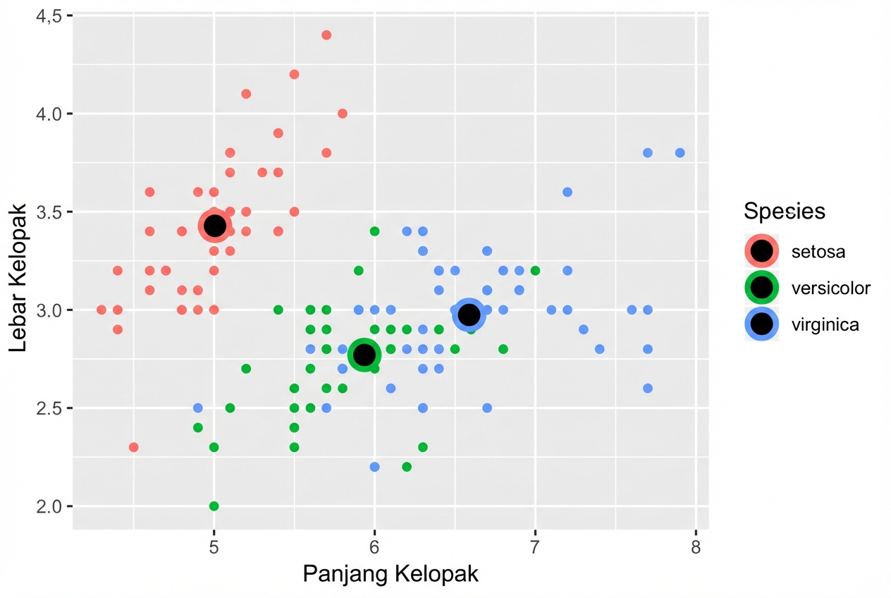
Kendalikan pemetaan estetika tiap layer secara independen:
ggplot(iris, aes(x = Sepal.Length, y = Sepal.Width, col = Species)) +
  # Mewarisi data dan aes dari ggplot()
  geom_point() +
  # Data berbeda, aes tetap diwarisi
  geom_point(data = iris.summary, shape = 15, size = 5)
Nilai atribut shape
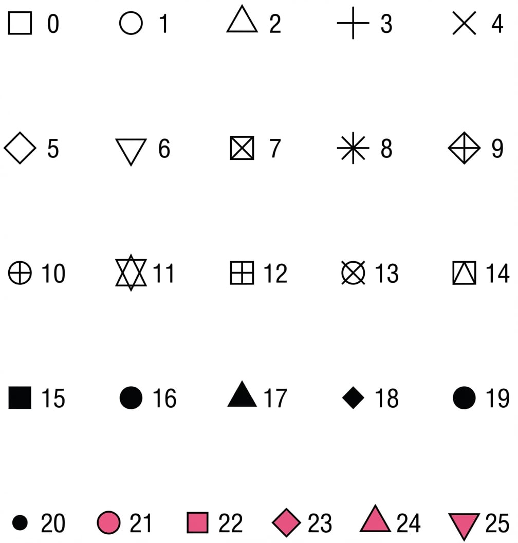
Contoh
ggplot(iris, aes(x = Sepal.Length, y = Sepal.Width, col = Species)) +
  geom_point() +
  geom_point(data = iris.summary, shape = 21, size = 5,
             fill = "black", stroke = 2)
Stat on-the-fly oleh ggplot2
- Lihat course kedua untuk layer stats.
- Catatan: Hindari memplot hanya mean tanpa ukuran sebaran, mis. standar deviasi.
position = "jitter"
ggplot(iris, aes(x = Sepal.Length, y = Sepal.Width, col = Species)) +
  geom_point(position = "jitter")
geom_jitter()
Cara singkat untuk geom_point(position = "jitter")
ggplot(iris, aes(x = Sepal.Length, y = Sepal.Width, col = Species)) +
  geom_jitter()
Jangan lupa atur alpha
- Gabungkan jitter dengan alpha-blending bila perlu
ggplot(iris, aes(x = Sepal.Length, y = Sepal.Width, col = Species)) +
  geom_jitter(alpha = 0.6)
Lingkaran kosong juga membantu
shape = 1adalah lingkaran kosong.- Tidak perlu juga pakai alpha-blending.
ggplot(iris, aes(x = Sepal.Length, y = Sepal.Width, col = Species)) +
  geom_jitter(shape = 1)