Confronta modelli AR e MA

Analisi delle serie temporali in R

David S. Matteson

Associate Professor at Cornell University

Processi MA e AR

  • Modello MA: $Oggi = Media + Rumore + Pendenza * (Rumore di ieri)$ $$Y_t = \mu + \epsilon_t + \theta\epsilon_{t-1}$$

  • Modello AR:

$(Oggi - Media) = Pendenza*(Ieri - Media)$ $$+ Rumore$$ $$Y_t - \mu = \phi(Y_{t-1} - \mu) +\epsilon_t$$

  • Dove:

$$\epsilon_t \sim WhiteNoise(0, \sigma^2_t)$$

Analisi delle serie temporali in R

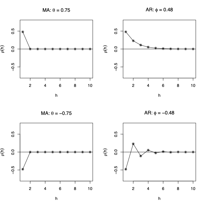
Processi MA e AR: autocorrelazioni

Analisi delle serie temporali in R

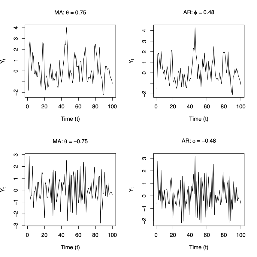
Processi MA e AR: simulazioni

Analisi delle serie temporali in R

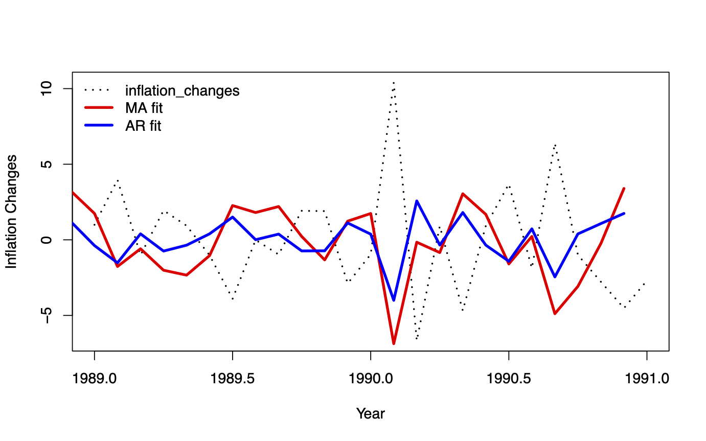
Processi MA e AR: valori adattati

  • Variazioni dell’inflazione USA mensile

Analisi delle serie temporali in R

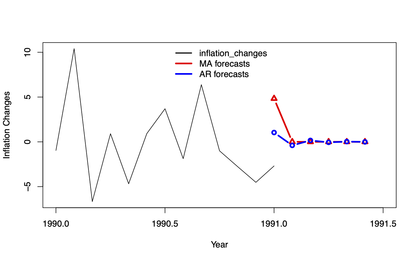
Processi MA e AR: previsioni

  • Variazioni dell’inflazione USA mensile

Analisi delle serie temporali in R
MA_inflation_changes <-
arima(inflation_changes, 
order = c(0,0,1))
         ma1 intercept
     -0.7932    0.0010
s.e.  0.0355    0.0281
sigma^2 estimated as 8.882: 
log likelihood = -1230.85, 
aic = 2467.7
AIC(MA_inflation_changes)
BIC(MA_inflation_changes)
2467.703
2480.286
AR_inflation_changes <- 
arima(inflation_changes, 
order = c(1,0,0))
         ar1 intercept
     -0.3849    0.0038
s.e.  0.0420    0.1051
sigma^2 estimated as 10.37: 
log likelihood = -1268.34, 
aic = 2542.68
AIC(AR_inflation_changes)
BIC(AR_inflation_changes)
2542.679
2555.262
Analisi delle serie temporali in R

Passons à la pratique !

Analisi delle serie temporali in R

Preparing Video For Download...