Modelli AR e MA

Modelli ARIMA in R

David Stoffer

Professor of Statistics at the University of Pittsburgh

Modelli AR e MA

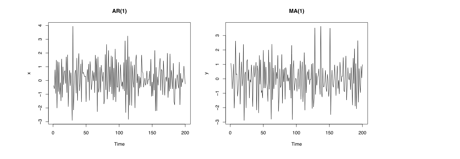
x <- arima.sim(list(order = c(1, 0, 0), ar = -.7), n = 200)
y <- arima.sim(list(order = c(0, 0, 1), ma = -.7), n = 200)
par(mfrow = c(1, 2))
plot(x, main = "AR(1)")
plot(y, main = "MA(1)")

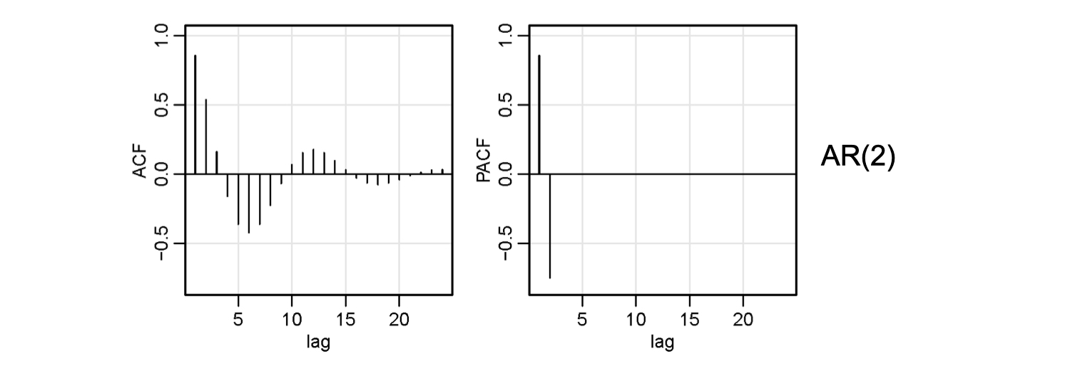
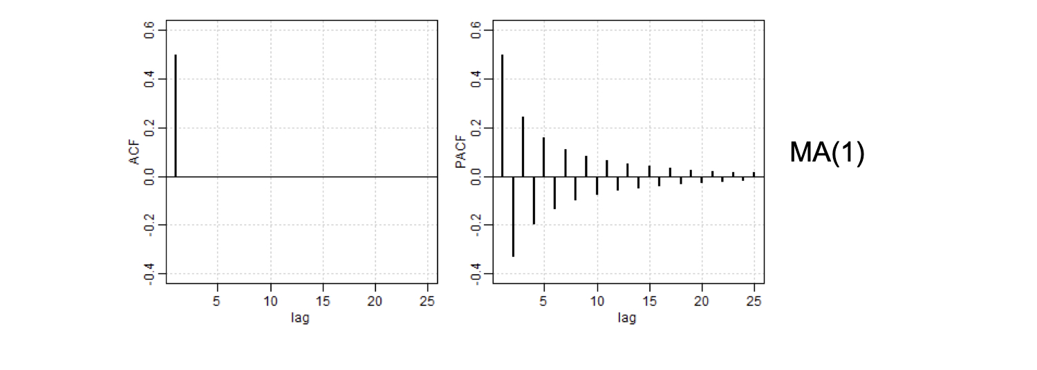
ch2_1.004.png

ACF e PACF

	AR(p)	MA(q)	ARMA(p, q)
ACF	Decresce	Si annulla al rit. q	Decresce
PACF	Si annulla al rit. p	Decresce	Decresce

ACF e PACF

	AR(p)	MA(q)	ARMA(p, q)
ACF	Decresce	Si annulla al rit. q	Decresce
PACF	Si annulla al rit. p	Decresce	Decresce

ch2_1.007.png

ACF e PACF

	AR(p)	MA(q)	ARMA(p, q)
ACF	Decresce	Si annulla al rit. q	Decresce
PACF	Si annulla al rit. p	Decresce	Decresce

ACF e PACF

	AR(p)	MA(q)	ARMA(p, q)
ACF	Decresce	Si annulla al rit. q	Decresce
PACF	Si annulla al rit. p	Decresce	Decresce

ch2_1.009.png

Stima

La stima per serie temporali è simile ai minimi quadrati in regressione
Le stime si ottengono numericamente con metodi di Gauss-Newton

ch2_1.013.png

Stima con astsa

AR(2) con media 50:

$$W_t = 50 + 1.5(X_{t-1} - 50) -.75(X_{t-2}- 50) + W_t $$

x <- arima.sim(list(order = c(2, 0, 0), 
                    ar = c(1.5, -.75)), 
                    n = 200) + 50
x_fit <- sarima(x, p = 2, d = 0, q = 0)
x_fit$ttable

      Estimate     SE  t.value p.value
ar1     1.5429 0.0435  35.4417       0
ar2    -0.7752 0.0434 -17.8650       0
xmean  49.6984 0.3057 162.5788       0

Stima con astsa

MA(1) con media 0:

$$X_t = W_t - .7W_{t-1}$$

y <- arima.sim(list(order = c(0, 0, 1), ma = -.7), n = 200)
y_fit <- sarima(y, p = 0, d = 0, q = 1)
y_fit$ttable

      Estimate      SE   t.value  p.value
ma1    -0.7459  0.0513  -14.5470   0.0000
xmean   0.0324  0.0191    1.6946   0.0917

Passiamo alla pratica !

Modelli ARIMA in R