Calcolare e descrivere le previsioni
Modelli lineari generalizzati in Python

Ita Cirovic Donev
Data Science Consultant
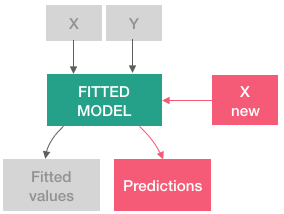
Calcolare le previsioni
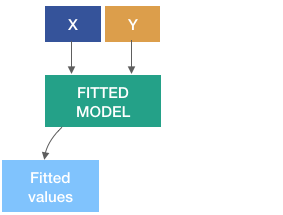
Calcolare le previsioni
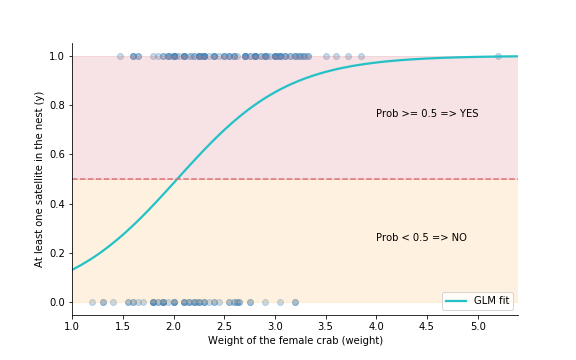
Da probabilità a classi
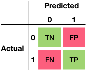
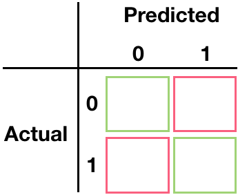
Matrice di confusione
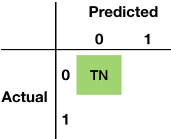
Matrice di confusione - Veri negativi
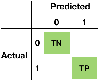
Matrice di confusione - Veri positivi
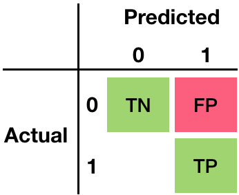
Matrice di confusione - Falsi positivi
Matrice di confusione - Falsi negativi