Metodi di shrinkage

Feature Engineering in R

Jorge Zazueta

Research Professor and Head of the Modeling Group at the School of Economics, UASLP

Due tecniche comuni di regolarizzazione

Lasso

Aggiunge una penalità proporzionale al valore assoluto dei pesi
Induce alcuni pesi a diventare esattamente zero
Elimina di fatto le rispettive feature
Può fungere da selezione automatica delle feature

Ridge

Aggiunge una penalità proporzionale al quadrato dei pesi
Non riduce alcuni coefficienti a zero come Lasso
Ma può ridurre efficacemente l'overfitting

Primo sguardo a Lasso

Imposta il modello

recipe <- # Define recipe
recipe(Loan_Status ~ ., data = train) %>%
  step_normalize(all_numeric_predictors()) %>% 
  step_dummy(all_nominal_predictors()) %>%
  update_role(Loan_ID, new_role = "ID")
# set up model
model_lasso_manual <- logistic_reg() %>%
  set_engine("glmnet") %>%
  set_args(mixture = 1, penalty = .2)
# Raggruppa nel workflow
workflow_lasso_manual <-
  workflow() %>%
  add_model(model_lasso_manual) %>%
  add_recipe(recipe)

Fitta e ispeziona

fit_lasso_manual <- # Fit workflow
  workflow_lasso_manual %>% 
  fit(train)
#Ispeziona i coefficienti
tidy(fit_lasso_manual)

# A tibble: 15 × 3
   term                    estimate penalty
   <chr>                      <dbl>   <dbl>
 1 (Intercept)               -0.816     0.2
 2 ApplicantIncome            0         0.2
 3 CoapplicantIncome          0         0.2
 4 LoanAmount                 0         0.2
 5 Loan_Amount_Term           0         0.2
 6 Credit_History            -0.220     0.2
 7 Gender_Female              0         0.2
 ...                          ...        ...

Logistica semplice vs. Lasso

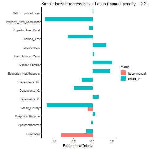
Grafico a colonne: regressione logistica semplice vs Lasso.

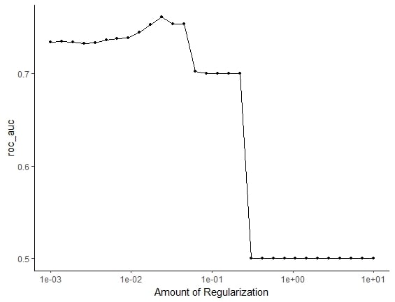
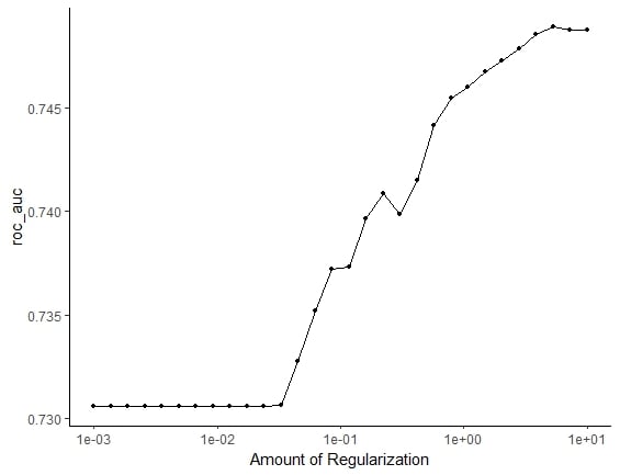
Tuning degli iperparametri

Impostare un modello con tuning

model_lasso_tuned <- logistic_reg() %>%
  set_engine("glmnet") %>%
  set_args(mixture = 1, 
  penalty = tune()) 

workflow_lasso_tuned <-
  workflow() %>%
  add_model(model_lasso_tuned) %>%
  add_recipe(recipe)

penalty_grid <- grid_regular(
  penalty(range = c(-3, 1)),
  levels = 30)

Esaminare l'output del tuning

tune_output <- tune_grid( 
  workflow_lasso_tuned,
  resamples = vfold_cv(train, v = 5),
  metrics = metric_set(roc_auc),
  grid = penalty_grid)
autoplot(tune_output)

Grafico di ROC_AUC rispetto alla quantità di regolarizzazione.

Esplorare i risultati

Caratteristiche selezionate automaticamente

best_penalty <- 
select_by_one_std_err(tune_output, 
metric = 'roc_auc', desc(penalty)) 

# Fit modello finale
final_fit<- 
finalize_workflow(workflow_lasso_tuned, 
best_penalty) %>%
  fit(data = train)

final_fit_se %>% tidy()

# A tibble: 15 × 3
   term                    estimate penalty
   <chr>                      <dbl>   <dbl>
 1 (Intercept)               -0.660  0.0452
 2 ApplicantIncome            0      0.0452
 3 CoapplicantIncome          0      0.0452
 4 LoanAmount                 0      0.0452
 5 Loan_Amount_Term           0      0.0452
 6 Credit_History            -0.948  0.0452
 7 Gender_Female              0      0.0452
 8 Married_Yes               -0.191  0.0452
 9 Dependents_X1              0      0.0452
10 Dependents_X2              0      0.0452
11 Dependents_X3.             0      0.0452
12 Education_Not.Graduate     0      0.0452
13 Self_Employed_Yes          0      0.0452
14 Property_Area_Rural        0      0.0452
15 Property_Area_Semiurban   -0.163  0.0452

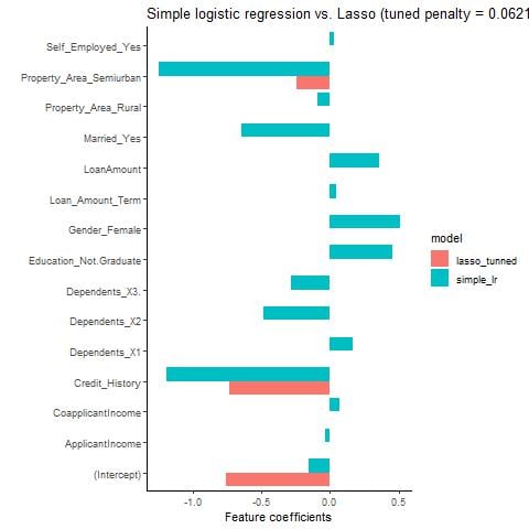
Logistica semplice vs. Lasso ottimizzato

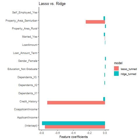
Regolarizzazione Ridge

Ridge è l'opzione con mixture = 0

model_ridge_tuned <- logistic_reg() %>%
  set_engine("glmnet") %>%
  set_args(mixture = 0, penalty = tune()) 

workflow_ridge_tuned <-
  workflow() %>%
  add_model(model_ridge_tuned) %>%
  add_recipe(recipe)

tune_output <- tune_grid( 
  workflow_ridge_tuned,
  resamples = vfold_cv(train, v = 5),
  metrics = metric_set(roc_auc),
  grid = penalty_grid)

tune_output <- tune_grid( 
  workflow_ridge_tuned,
  resamples = vfold_cv(train, v = 5),
  metrics = metric_set(roc_auc),
  grid = penalty_grid)  
 autoplot(tune_output)

Regolarizzazione Ridge

best_penalty <- 
select_by_one_std_err(tune_output,
metric = 'roc_auc', desc(penalty)) 
best_penalty

final_fit<- 
finalize_workflow(workflow_ridge_tuned, 
best_penalty) %>%
  fit(data = train)

tidy(final_fit)

# A tibble: 15 × 3
   term                      estimate penalty
   <chr>                        <dbl>   <dbl>
 1 (Intercept)             -0.799          10
 2 ApplicantIncome          0.00232        10
 3 CoapplicantIncome        0.0000537      10
 4 LoanAmount               0.00291        10
 5 Loan_Amount_Term         0.00161        10
 6 Credit_History          -0.0245         10
 7 Gender_Female            0.00850        10
 8 Married_Yes             -0.0140         10
 9 Dependents_X1            0.00497        10
10 Dependents_X2           -0.0100         10
11 Dependents_X3.           0.00259        10
12 Education_Not.Graduate   0.00308        10
13 Self_Employed_Yes        0.00892        10
14 Property_Area_Rural      0.0109         10
15 Property_Area_Semiurban -0.0139         10

Ridge vs. Lasso

Mettiamoci alla prova!

Feature Engineering in R